Making sense of LSTMs by example
TL;DR
After reading Andrej Karpathy’s blog on recurrent neural nets (RNN) in general and Christopher Olah’s blog about long short-term memory networks (LSTM), I decided to add some “intuitive” examples to illustrate the roles of the cell and hidden states as well as the different gates in an LSTM.
Recurrent Neural Networks with Memory
Recurrent neural networks (RNN) with memory can do amazing feats when trained to predict the next character in a text sequence, as Andrej Karpathy demonstrates in this nice article. Instead of learning a plain function that maps inputs to outputs (such as recognizing a digit in an image or telling whether there is a cat on it) these models carry memory with them.
Imagine yourself typing In France, I ate ... or In Italy, I ate .... You’d probably be much more inclined to bet on croissant, baguette, or cheese in the first case and pizza, pasta, or bruschetta in the second case. State matters. More precisely, a summary of what you have already seen in the past.
While the recurrent in RNNs suggests that feeding back the output of hidden layer into its input is central, I think the “memory-update” part is even more important. In the previous example, think of a little “France” LED getting activated whenever something France-related is read in the input. Later on, I can rely on this “bookmarked” information and the current input to make guesses about the next word. Consider a turnstile for an analogy:
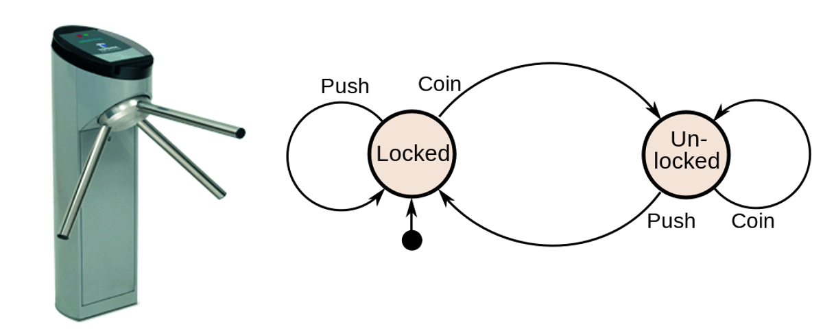
The turnstile will react differently to the input push, depending on whether it was in the state unlocked (after receiving its well-deserved coin) or not - just as you’d expect! Fascinatingly, RNNs will figure out which states and “state transition logic” they need to accomplish the task they are trained on (e.g., predicting the next character or word). The states will typically not be as clean and easy to interpret but rather messy vectors [0.1, -0.7, 1.2] and matrix multiplications with non-linearities to represent the transitions. If you’re feeling confused or lost at this point, read Karpathy’s blog to brush up on the inner workings of RNNs.
But first, let’s make really explicit what it means for a neural network to “store” information in memory (and to read from it).
Reading and writing into memory as operations in a neural network
For the sake of the argument, assume that our turnstile expects two coins, one euro each, in order to open.
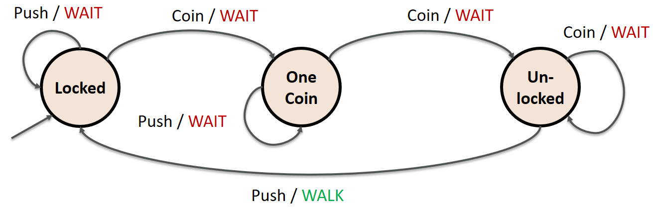
In a sense, the “memory” is just a vector of numbers and storing/reading are matrix operations with non-linearities (e.g., ReLU). For example, let us assume that we have a two-dimensional memory vector: \(\begin{align} h &= \begin{bmatrix} 2 \\ 0 \end{bmatrix} \end{align}\) where the first component (here 2) represents the number of coins already inserted and the second component (here 0) stores how many times we have already passed the turnstile. We can picture our turnstile using these states as follows:
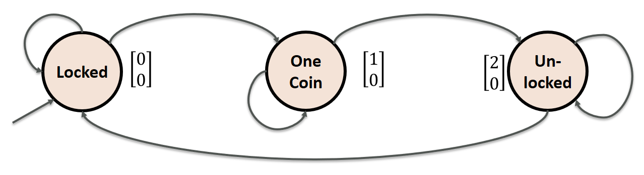
Our intuition should be that outputting “WALK” is only feasible if we’re in state \(\begin{bmatrix} 2 \\ 0 \end{bmatrix}\). And we can only get to that state by reading “coin” twice!
Now, how should we express storing information? For example, when reading the input “coin”, we want to increment the first component of \(h\). Let’s represent “coin” and “push” as vectors first:
\[c = \begin{bmatrix} 1 \\ 0 \end{bmatrix} \quad p = \begin{bmatrix} 0 \\ 1 \end{bmatrix}\]Our task is to come up with an operation that, given memory state \(\begin{align} h &= \begin{bmatrix} 0 \\ 0 \end{bmatrix} \end{align}\), returns \(\begin{align} \begin{bmatrix} 1 \\ 0 \end{bmatrix} \end{align}\) and, similarly, maps \(\begin{align} \begin{bmatrix} 1 \\ 0 \end{bmatrix} \end{align}\) to \(\begin{align} \begin{bmatrix} 2 \\ 0 \end{bmatrix} \end{align}\) but only if the input is $c$ (for “coin”). To put this in “neural-network-friendly” terms, we want to express this using a matrix multiplication (ignoring bias to keep it simple) and an activation function (we use ReLU).
\[h_{t+1} = f_W(h_t, x_t) = \max\{0, W_{hh} h_{t} + W_x x_t\}\]We (or our network in training) need to tweak the matrices $W_{hh}$ and $W_{x}$ such that
\[f_W( \underbrace{ \begin{bmatrix} 0 \\ 0 \end{bmatrix} }_{h_{t}}, \underbrace{\begin{bmatrix} 1 \\ 0 \end{bmatrix}}_c) = \underbrace{\begin{bmatrix} 1 \\ 0 \end{bmatrix}}_{h_{t+1}} \qquad f_W( \underbrace{ \begin{bmatrix} 1 \\ 0 \end{bmatrix} }_{h_{t}}, \underbrace{\begin{bmatrix} 1 \\ 0 \end{bmatrix}}_c) = \underbrace{\begin{bmatrix} 2 \\ 0 \end{bmatrix}}_{h_{t+1}}\]Fortunately, for that simple task, we could set $W_{hh}$ and $W_{x}$ to be the identity $I$ to make the calculations work out fine (we’ll take care of more complications later).
\[\max\{0, \begin{bmatrix} 1 & 0 \\ 0 & 1 \end{bmatrix}\begin{bmatrix} 0 \\ 0 \end{bmatrix} + \begin{bmatrix} 1 & 0 \\ 0 & 1 \end{bmatrix} \begin{bmatrix} 1 \\ 0 \end{bmatrix} \} = \begin{bmatrix} 1 \\ 0 \end{bmatrix}\] \[\max\{0, \begin{bmatrix} 1 & 0 \\ 0 & 1 \end{bmatrix}\begin{bmatrix} 1 \\ 0 \end{bmatrix} + \begin{bmatrix} 1 & 0 \\ 0 & 1 \end{bmatrix} \begin{bmatrix} 1 \\ 0 \end{bmatrix} \} = \begin{bmatrix} 2 \\ 0 \end{bmatrix}\]Long short-term memory
A particularly famous extension is the LSTM network, the long short-term memory network by Jürgen Schmidhuber and Sepp Hochreiter.
LSTMs implement essentially the same logic as an RNN with memory in a more gradient-friendly manner. Christopher Olah described the inner workings of the LSTM in a beautiful blog article. There are many posts dealing with their training dynamics but I want to focus on an instructive example to make sense of the components.
That is a lot of calculations compared to a vanilla RNN!
Why do LSTMs have all these gates and recurrent connections?
The short answer is, it seems not to be completeley well understood. This paper by Google made an extensive effort to find better architectures (also by random mutations and evolutionary search) but basically did not find anything substantially worse or better.
Let’s first work with an incredibly stereotypical but illustrative sentence:
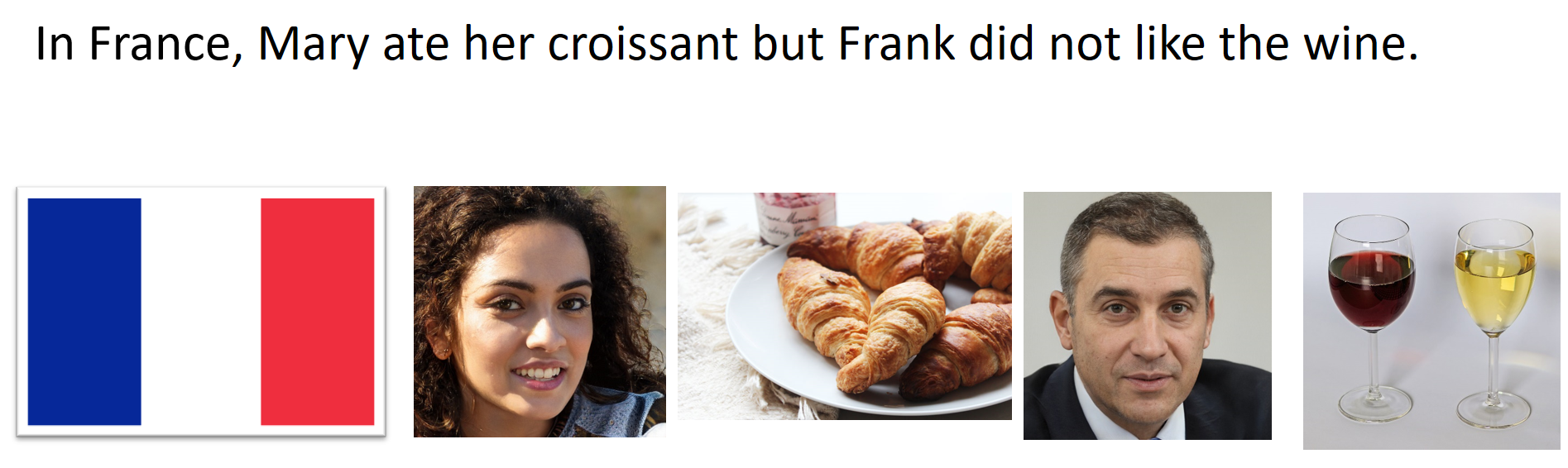
Intuitively, when we are at the position of “her”, we would know it’s about eating, a female person, and France – naturally, croissant would make sense as a next guess! (btw, don’t worry about Mary’s and Frank’s picture being used, they do not exist).
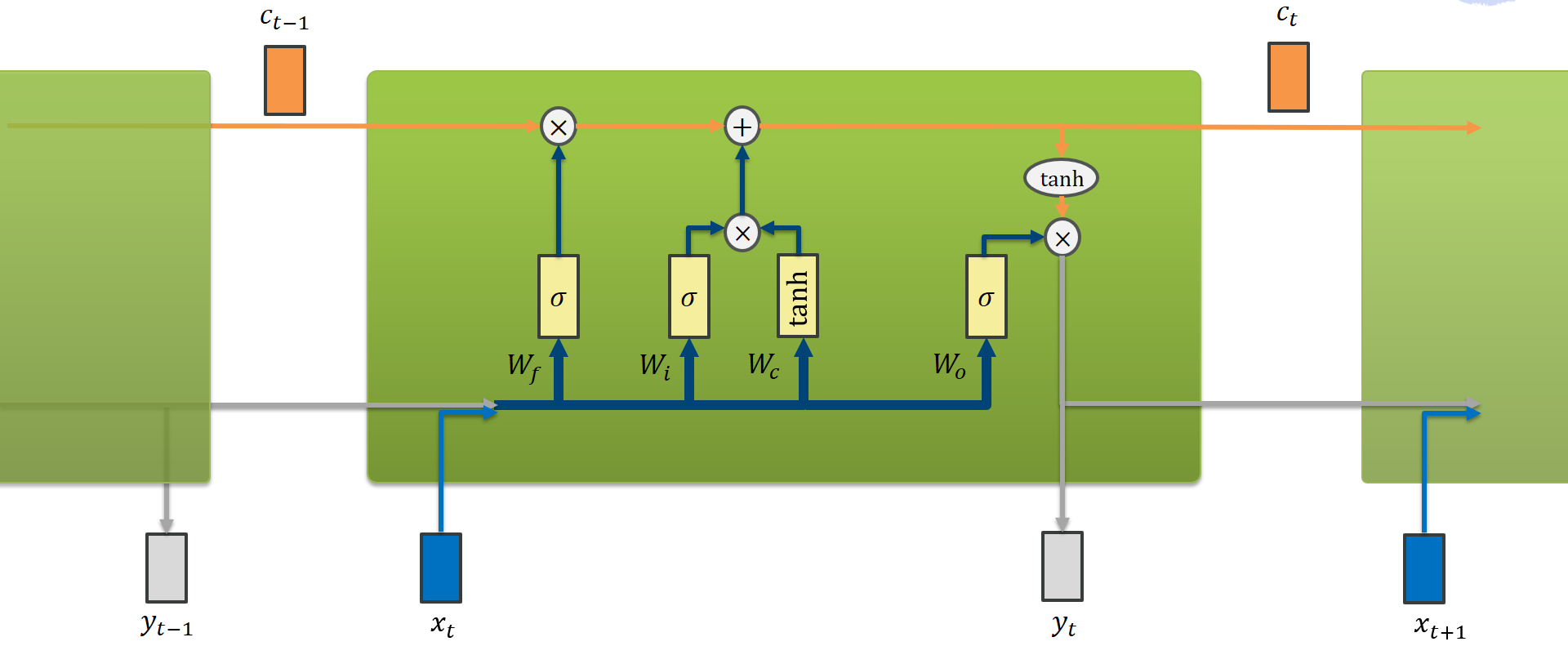
We will walk through all gates (input gate, forget gate, and output gate) using that sentence. The calculations can be thought of as follows:
The individual features in the hidden cell state do not necessarily bear any clear interpretable meaning. But for our purposes, suppose they are arranged like this:
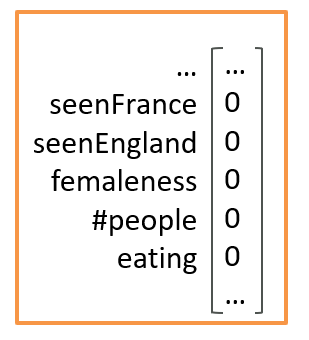
Note that we can have more “boolean” features like the flag indicating whether we have seen France in the sentence or not, but also numerical features such as the number of people in the sentence. Updates to the cell state are not constrained to lie between 0 and 1.
The input phase
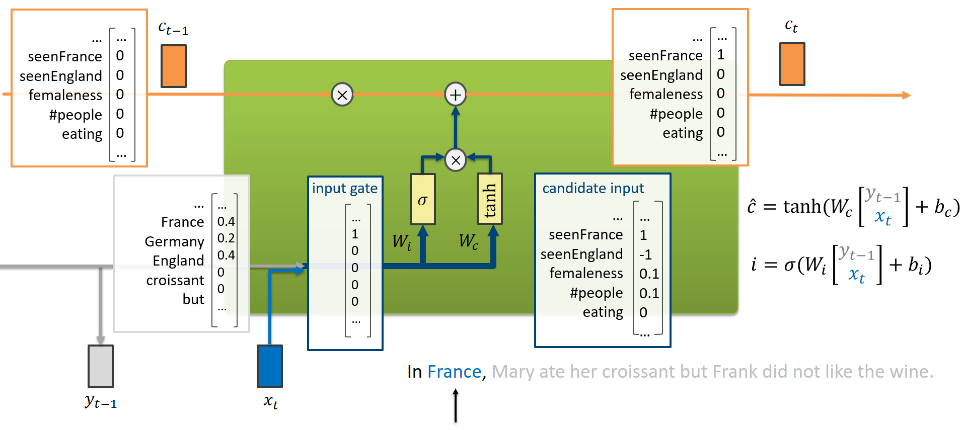
Suppose we just read “France”. That means, the previous output of our model was based on reading “In”, so it was probably more inclined to output “France”, “Germany”, or “England” than words like “but” or “croissant”. That is represented by $y_{t-1}$.
That information is concatenated with the current input $x_t$ to form just a stacked vector. Our model has learned to produce a setting for the input gate (which information may pass through to the cell state) based on $(y_{t-1}, x_t)$, using the weight matrix $W_i$. In this example, it decided (rightfully) to open the information gate for the feature seenFrance.
Somewhat in parallel, it also produces a “candidate” input $\hat{c}$ that contains the tentative updates to the cell state. Here, our model would like to crank up the Frenchiness and reduce the Englishness in our cell state. But the input gate decided not to care about other features than the Frenchiness.
This seems very confusing and redundnant work. But essentially, it simply adds another piece of nonlinearity (hence flexibility) for the network’s update functions. Do not ascribe too much meaning to it!
Finally, our cell state $c_t$ has toggled its seenFrance feature.
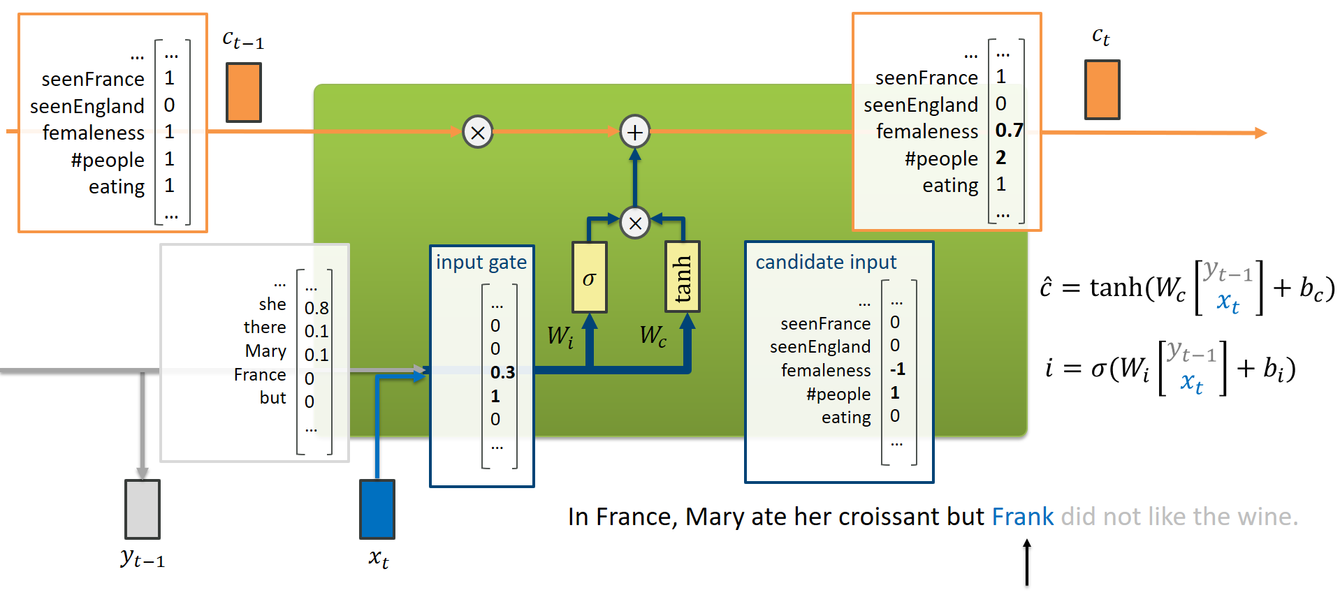
In a similar vein, we could imagine what happens when we read “Frank”:
The forget phase
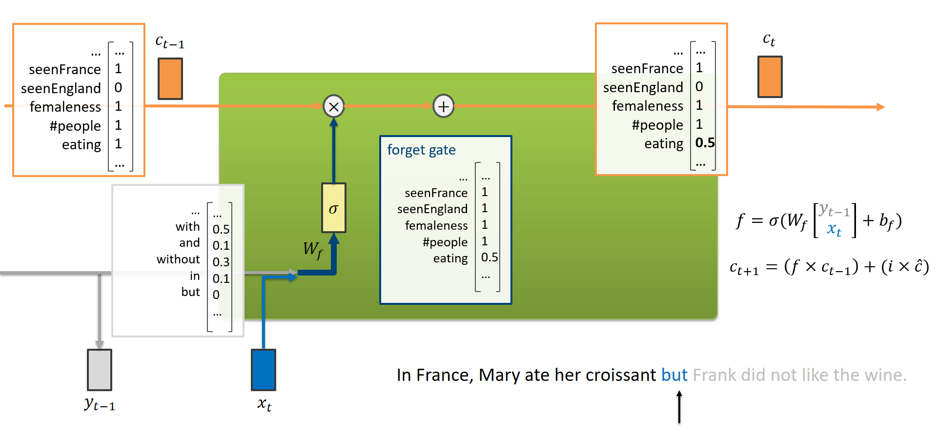 Forgetting follows a simpler flow than memorizing (in fact, the forget gate was not part of the original LSTM by Hochreiter and Schmidhuber). Again, the LSTM concatenates $(y_{t-1}, x_t)$ and decides the positions of the forget gate (using the trained weights $W_f$) which is simply multiplied with the cell state. Values close to 1 mean “just keep the state as it is”, values close to 0 mean “erase that state from our memory”.
When reading “but”, our network might have learned that the activity of eating is not as relevant to the context of the sentence as it used to be.
The output phase
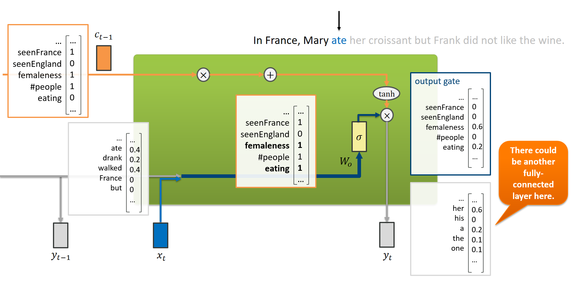
Finally, we also want our LSTM to produce an output that can be matched to a target during training. Depending on the application (sequence to sequence, vector to sequence, etc.), we may or may not consider every output of the network.
The LSTM uses the updated cell state $c_t$ to produce an output $y_t$, using the output gate. The latter is again a gate setting resulting from a learned weight matrix $W_o$.
When reading “ate”, the LSTM must have updated the cell state in such a way that now it can produce an output that now is likely to be her since we have seen a female person earlier on. (The interpretability of the cell states towards the output features that are matched to targets is a bit lost at this point.)
Conclusion
Long short-term memory networks provide a clever arrangement of gates and connections that improve the gradient flow. The inner workings may be a bit hard to conceptualize - but fortunately we do not really have to do that, as long as our networks work well. I hope this post is useful to at least convey the idea that it can work.
Real LSTM cells are much harder to interpret and understand. But LSTMVis provides a really nice tool to play around with and appreciate the complexity encoded in these networks. Give it a go!