Automatic Differentiation for Deep Learning, by example

TL;DR

In essence, neural networks are simply mathematical functions that are composed of many simpler functions. During training, we need to find partial derivatives of each weight (or bias) at a specific weight setting to make adjustments. All partial derivatives together are called the gradient (vector) and boil down to real numbers for a specific input to the function. This calculation can be easily programmed using reverse mode automatic differentiation which powers numerical frameworks such as TensorFlow or PyTorch. Let’s peek under the hood and work out a couple of concrete examples (including a small Numpy implementation) to see the magic and connect the dots!

Find a jupyter notebook accompanying the post here or directly in Colab:

Run in Google Colab

Understanding the Chain Rule

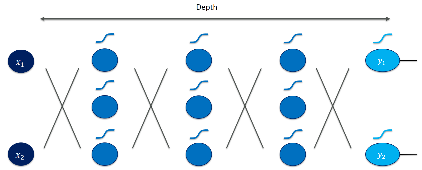
Neural networks calculate their output (for a given input) by repeatedly multiplying features by weights, summing them up, and applying activation functions to obtain non-linear mappings.

Especially in very deep networks (e.g., ResNet152 has 152 layers!), calculating the partial derivatives for the weight updates seems daunting and error-prone to do manually.

At this point of studying backpropagation, I was severely nervous about taking all those derivatives by hand … Fortunately, this tedious procedure is a mechanical operation that we can easily automate - at least for certain concrete values of a function (as opposed to getting a nice and clean symbolic function such as “$2x$” for “$x^2$” that we do not even need for training neural networks)!

A major source of confusion to me was the "data type" of a gradient or the partial derivatives, for that matter. In my mind, the meaning of df / dt was a 'function', as in "the function over all of its domain", perhaps in symbolic form. But here, we refer to specific value of the gradient at a specific point, i.e., a set of weights with concrete values, say [0.4, 1.2]. Because that's really all we need for training!

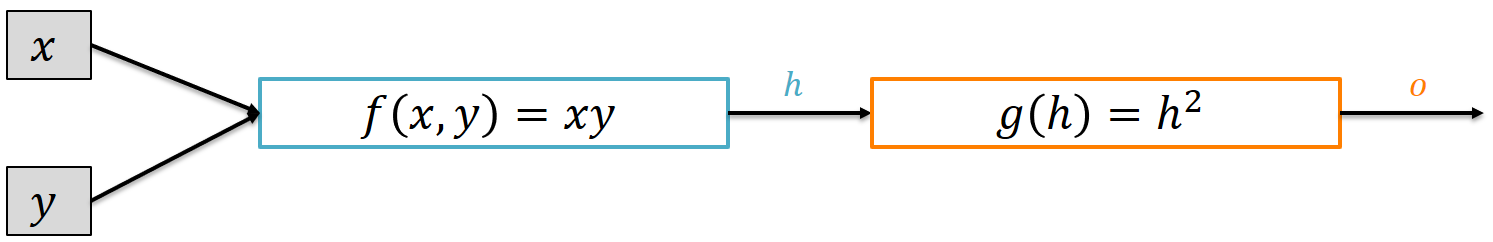
Since neural networks chain together several weighted sums and activation functions we need to revisit the chain rule (again, 3Blue1Brown saves the day!). We are moving from neural networks such as $f(\vec{w}; \vec{x}) = \max ( \sum_{i = 1}^k w_i \cdot x_i, 0)$ to much simpler functions, for the moment. A very helpful picture to visualize is that of a computational graph as a circuit of functions with input and output values that are chained together, as proposed by CS231n.

Or in code:

def f(x,y):
    return x*y

def g(h):
    return h**2

h = f(3,2)
o = g(h)

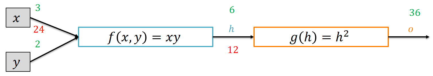
The input values $x$ and $y$ are fed into the first function $f$ (which just multiplies them together) to form the intermediate variable $h$ which is then fed into $g$ to form the output $o$. Let’s apply this to the inputs 3 and 2:

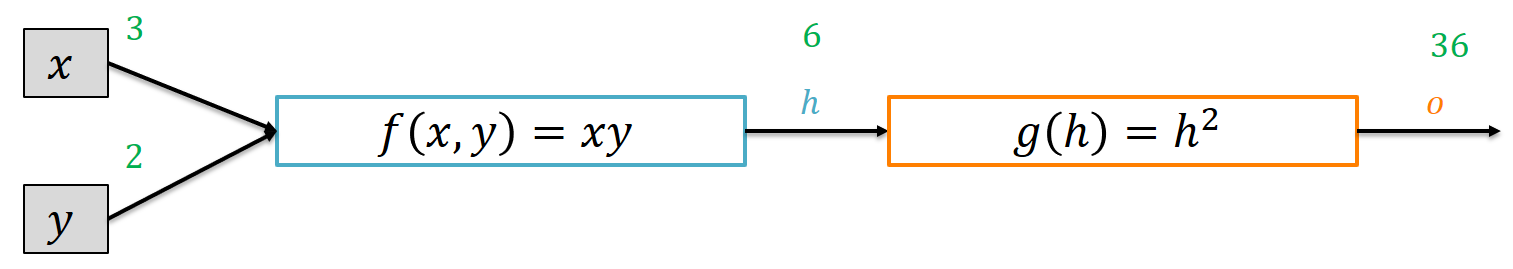
We can view $o$ as a function of $x$ and $y$ which makes it natural to ask for its partial derivatives, $\frac{\partial o}{\partial x}$ and $\frac{\partial o}{\partial y}$. This perspective gives a very intuitive interpretation of the chain rule. Being a bit sloppy here (mathematically), think of the partial derivative $\frac{\partial o}{\partial h}$ as the ratio between the change in $o$ that a little nudge to $h$ provokes.

Let’s work this out in isolation for both functions. Consider $x = 3$ and $y = 2$. Differentiating according to $x$ yields $\frac{\partial h}{\partial x} = y$, for the concrete case 2. That means that a little increment to $x$ such as 0.01 would provoke a change by a factor 2, so $h$ would increase by 0.02.

Similarly, for $h = 6$ the derivative of $g(h) = h^2$ (of course, with respect to $h$) yields $2h$, 12 for our example. Hence, increasing $h$ by 0.01 would cause an increase by 0.12 in $o$. Now just chain these two together: A little increase $\Delta$ in $x$ will trigger a $2\Delta$ increase in $h$. And since every $\Delta$ increase in $h$ causes a $12\Delta$, the total increase in $o$ when we increase $x$ by $\Delta$ is simply $2 \cdot 12 \cdot \Delta$, i.e., a factor of $24$. Although this thought is not formally bullet-proof (we’re dealing with limits and such) it helped me a lot to form intuition and the arithmetic of the chain rule is consistent with it:

\[\frac{\partial o}{\partial x} = \frac{\partial o}{\partial h} \cdot \frac{\partial h}{\partial x}\]

which we can again program exactly for given values of $x$ and $y$:

x,y = 3,2
h = f(x,y) 
o = g(h)

# first the partial derivative d o / d h
do_dh = 2*h
>>> 12
dh_dx = y
>>> 2 
# then the chain rule application
do_dx = do_dh * dh_dx
>>> 24

which we can use to fill in our graph diagram:

If we apply the chain rule for $y$, we get an analogous result:

\[\frac{\partial o}{\partial y} = \frac{\partial o}{\partial h} \cdot \frac{\partial h}{\partial y}\]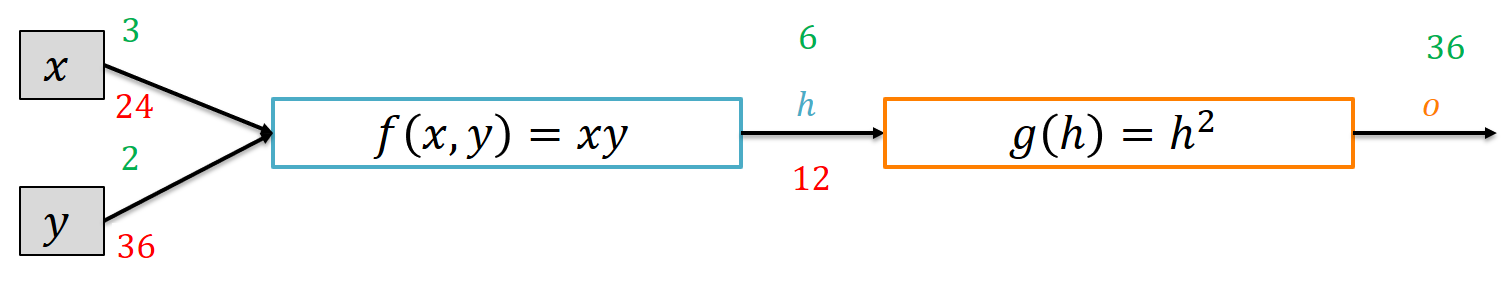

Note that the partial derivative $\frac{\partial o}{\partial y}$ is simply larger because we multiply $\frac{\partial o}{\partial h} = 12$ by $\frac{\partial h}{\partial y} = 3$, every increase in $y$ is multiplied by $x = 3$.

But, more importantly, note that $\frac{\partial o}{\partial h} = 12$ appears in both calculations!

That is a key observation that is also exploited in backpropagation for neural networks: We can reuse derivatives for shared subexpressions in the gradient calculation, if we schedule the calculations correctly: Work out derivatives of the later layers before those of the earlier layers and reuse the results. Doing that in the right order is called the backward pass of a neural network, for apparent reasons:

The calculation needs the intermediate values (here, $h$) to calculate the partial derivatives and has to calculate them in the reverse order of the forward computation (this is why this method is called reverse mode automatic differentiation).

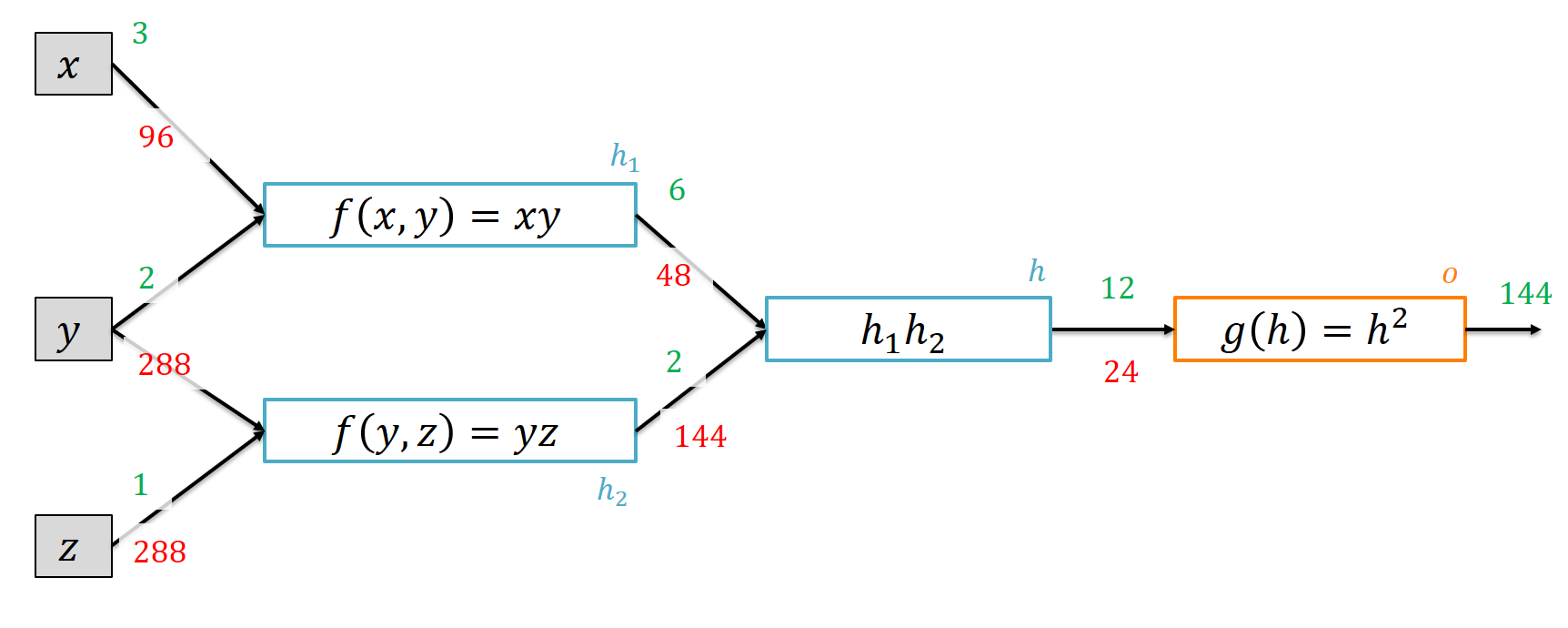
We can also look at somewhat more entangled graphs:

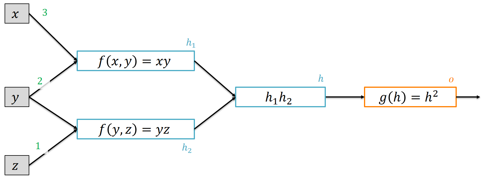
where, again, every subexpression gets their own name. Go ahead and try to perform forward and backward calculation using the chain rule!

You might have noticed that the variable $y$ affects the output $o$ via two paths: Once when calculating $h_1$, once for $h_2$. Fortunately, it suffices to sum up all effects that $y$ has to get the overall effect on $o$. Mathematicians call this the multivariable chain rule. We need this in neural networks since changing a weight in early layers affects multiple hidden units and outputs - and finally the loss.

Now we observe a pattern that makes the whole process look very algorithmic, i.e., easy to automate for a computer. Simple functions are chained together to form more complex functions and we can calculate all partial derivatives in one go by simple reversing the order of operations. Notice how all we needed to do to calculate these derivatives were just a couple of multiplications and additions - this is what makes GPUs so good for training neural nets! I think that is really cool.

Dynamic computation graphs and automatic differentiation

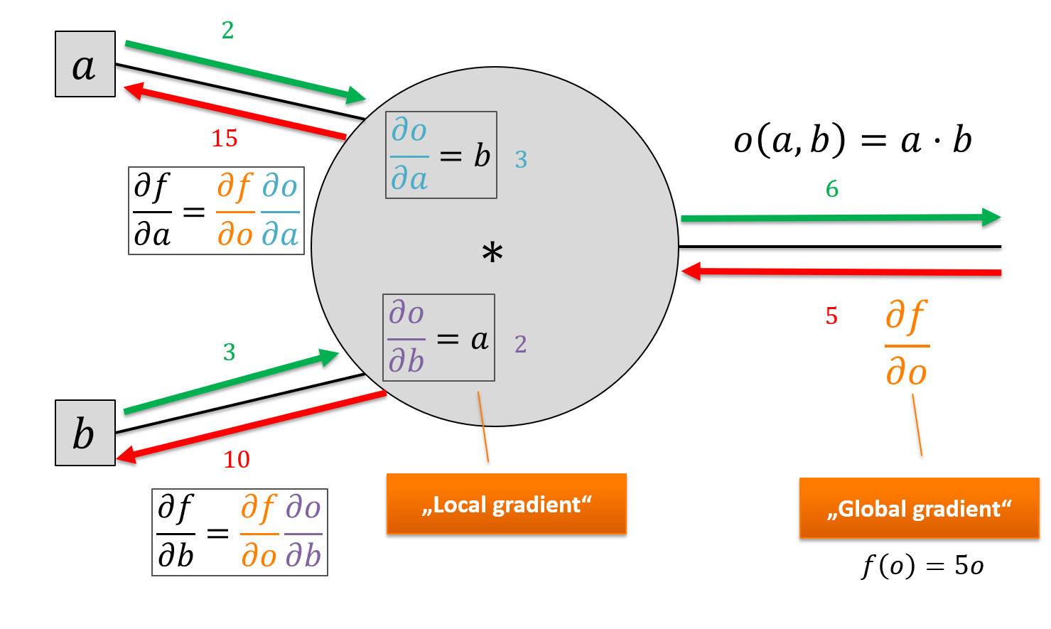
A single computational node (e.g., for multiplying or adding or taking the square) only has to perform the operation, store its output and know how to take the local derivative, given the derivative of its output. Let’s zoom in on such a guy:

For now, we only care about scalar functions (i.e., a single number) as the output of our computational graph. To calculate the partial derivatives, we have to do the local chain-rule updates in the reverse order of the forward calculations. Every node thus gets a gradient attribute for its output (the red numbers). That way, we can be sure that any “upstream gradient” is calculated before we need it in downstream nodes.

A general solution would be to calculate the graph in forward order and then perform topological sorting to find an appropriate linear ordering. Conceptually even simpler are gradient tapes. We might think of keeping a “log” like this:

#1: h1 = Multiply(3,2)
#2: h2 = Multiply(2,1)
#3: h = Multiply(h1, h2)
#4: o = Square(h)

and reversing the order of operations when calculating the derivatives

#4: grad o = Square(h)
#3: grad h = Multiply(h1, h2)
#2: grad h2 = Multiply(2,1)
#1: grad h1 = Multiply(3,2)

Our implementation revolves around the base class CompNode from which all our concrete functions (multiplication, squaring, adding, etc.) would inherit (an example of the composite pattern):

class CompNode:
    def __init__(self, tape):
        # make sure that the gradient tape knows us
        tape.add(self)
    
    # perform the intended operation 
    # and store the result in self.output
    def forward(self):
        pass
    
    # assume that self.gradient has all the information 
    # from outgoing nodes prior to calling backward
    # -> perform the local gradient step with respect to inputs
    def backward(self):
        pass
    
    # needed to be initialized to 0 
    def set_gradient(self, gradient):
        self.gradient = gradient
        
    # receive gradients from downstream nodes     
    def add_gradient(self, gradient):
        self.gradient += gradient

The gradient tape does little more than expect computation nodes, store their order of operations, and call backward on every computation node in the reverse order:

class Tape:    
    def __init__(self):
        self.computations = []
        
    def add(self, compNode : CompNode):
        self.computations.append(compNode)
        
    def forward(self):
        for compNode in self.computations:
            compNode.forward()
            
    def backward(self):
        # first initialize all gradients to zero 
        for compNode in self.computations:
            compNode.set_gradient(0)
            
        # we need to invert the order    
        self.computations.reverse()    
        # last node gets a default value of one for the gradient
        self.computations[0].set_gradient(1)
        for compNode in self.computations:
            compNode.backward()

The last node (our overall scalar output) receives a gradient of one (since $\frac{\partial f}{\partial f} = 1$).

A particular simple node is that representing a constant value.

class ConstantNode(CompNode):
    def __init__(self, value, tape):
        self.value = value
        super().__init__(tape)
        
    def forward(self):
        self.output = self.value
    
    def backward(self):
        # nothing to do here
        pass

which we can use for a and b

t = Tape()
a = ConstantNode(2,t)
b = ConstantNode(3,t)

The multiplication operation is rather straightforward to implement:

class Multiply(CompNode):
    
    def __init__(self, left : CompNode, right : CompNode, tape : Tape):
        self.left = left
        self.right = right
        super().__init__(t)
        
    def forward(self):
        self.output = self.left.output * self.right.output
        
    # has to know how to locally differentiate multiplication
    def backward(self):
        self.left.add_gradient(self.right.output * self.gradient)
        self.right.add_gradient(self.left.output * self.gradient)

Note that it stores references to its inputs (left and right) in order to inform them about gradients. In the forward pass, it simply multiplies the outputs of both input nodes and stores this as its own output. In the backward pass, it multiplies each input’s gradient with the opposite input’s output. Is that a bug?

No, it’s simply the local gradient for multiplication: if $f(a,b) = a \cdot b$ then $\frac{\partial f}{\partial a} = b$ and $\frac{\partial f}{\partial b} = a$ and those are exactly the local gradients we need!

We are now ready to automatically differentiate our previous example:

t = Tape()
a = ConstantNode(2,t)
b = ConstantNode(3,t)

o = Multiply(a, b, t)
f = Multiply(ConstantNode(5, t), o, t)
t.forward()

Calling backward on the tape will trigger the reverse-mode automatic differentiation. Some people call already that step backpropagation which I would reserve for the application of autodiff to neural networks and applying a gradient update on the weights.

t.backward()
print(o.gradient)
>>> 5
print(a.gradient) 
>>> 15
print(b.gradient)
>>> 10

Equipped with multiplication alone, we can even address our previous diamond-shaped graph:

t = Tape()
x = ConstantNode(3,t)
y = ConstantNode(2,t)
z = ConstantNode(1,t)

h1 = Multiply(x, y, t)
h2 = Multiply(y, z, t)

h = Multiply(h1, h2, t)
o = Multiply(h, h, t)
t.forward()

which replaced squaring by multiplication with itself.

t.backward()
print(h.gradient)
>>> 24 
print(h1.gradient)
>>> 48
print(h2.gradient)
>>> 144
print(x.gradient)
>>> 96
print(y.gradient)
>>> 288
print(z.gradient)
>>> 288

How would you implement the squaring operation ($x^2$) more explicitly? The forward operation is rather obvious: we have one input and take the square as the node’s output. What about the backward operation? If our input is $x$ and our output is $f(x) = x^2$ then the local gradient is simply $\frac{\partial f}{\partial x} = 2\cdot x$ where $x$ is the input to the node.

class Square(CompNode):
    
    def __init__(self, x : CompNode, tape : Tape):
        self.x = x
        super().__init__(t)
        
    def forward(self):
        self.output = self.x.output**2
        
    # has to know how to locally differentiate x^2
    def backward(self):
        self.x.add_gradient( (2*self.x.output) * self.gradient)

and applying it is then rather straightforward:

t = Tape()
x = ConstantNode(3,t)
y = ConstantNode(2,t)
z = ConstantNode(1,t)

h1 = Multiply(x, y, t)
h2 = Multiply(y, z, t)

h = Multiply(h1, h2, t)
o = Square(h, t)
t.forward()

Verify for yourself that this yields the same gradients! Why would you even do this if you can express squaring by multiplication? Well, sometimes the gradient expressions are substantially simplified algebraically, as is the case for the sigmoid function $f(z) = \frac{1}{1 + e^{-z}}$. It has a nice local derivative $\frac{\partial f}{\partial z} = f(z) \cdot (1 - f(z))$ which can be expressed only in terms of the node’s output. Or you could implement every step using a primitive operation (see CS231n course notes for an example). Your call! The general heuristic is “if there is an algebraically nice derivative (sigmoid, softmax), implement a CompNode for it, otherwise just let the framework work it out”.

As an exercise, try to implement the Add operation for simple addition. You can imagine building up an extensible autodiff framework with functions as building blocks that come with their own logic to differentiate – that’s precisely what deep learning frameworks do (among other cool things such as GPU-support, distributed execution, and pre-defined higher-level abstractions such as “layers” for neural nets)!

But why don’t TensorFlow or PyTorch look so complicated?

Admittedly, the way we wrote down reverse-mode autodiff with a gradient tape looks very tedious and unintuitive. You have all these objects for calculations and have to chain them together in the right way instead of writing arithmetic expressions such as:

o = ( (x*y) * (y * z) )**2

What if I told you you can have the cake and eat it, too? The key ingredient here is operator overloading.

When you write

a * b 

the return type of this expression (and even the function that works on a and b) depends on the types of the arguments. If a and b are normal int values, standard multiplication is used. If a and b are instances of CompNode we could go on and define or own version of *, e.g., one that takes both arguments to the constructor of our class Multiply. But be aware that you’re essentially defining calculations at this point (in PyTorch, you also get the forward pass immediately) instead of only executing them!

This helps to build a framework that has a nice frontend language to define calculations but handle the bookkeeping (wiring of operations, scheduling backward passes) in the background, without your noticing. Pretty neat, eh?

Under the hood, that is what powers PyTorch or TensorFlow:

x = tf.constant(3.0)
with tf.GradientTape(persistent=True) as t:
  t.watch(x)
  y = x * x
  z = y * y
dz_dx = t.gradient(z, x)  # 108.0 (4*x^3 at x = 3)
dy_dx = t.gradient(y, x)  # 6.0
del t  # Drop the reference to the tape

Connecting dots with Neural Networks

Well, we have worked through an algorithmic approach to differentiating composed functions. Essentially this saves us trouble when applying the chain rule by calculating intermediate derivatives that we need for the derivatives we actually care about.

But what does that have to do with a neural network?

Consider a single training instance $(\vec{x}, \vec{t})$ where $\vec{x} = [x_1, x_2, \ldots, x_m]$ and $\vec{t} = [t_1, \ldots, t_d]$. Our neural network transforms $\vec{x}$ to some output $\vec{y} = [y_1, \ldots, y_k]$ that can be compared to the target (what the network should produce) using its current set of weights. Let’s make this more explicit:

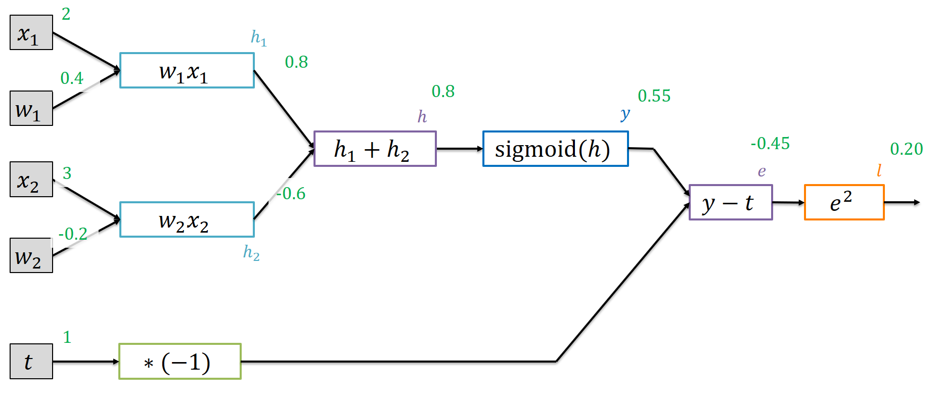
For the inputs $\vec{x} = (2,3)$, the network with its current weights $0.4$ and $-0.2$ produces a scalar output $y$ using the sigmoid activation function. It outputs $0.55$ but we would like that to be closer to $1$ (the target $t$). As loss function, the squared error measures how far we are off. We can implement this graph using a few additional CompNode extensions (that you can find in the notebook).

gt = Tape()
x1 = ConstantNode(2.,gt)
w1 = ConstantNode(0.4,gt)
x2 = ConstantNode(3.,gt)
w2 = ConstantNode(-0.2,gt)
t = ConstantNode(1.,gt)

h1 = Multiply(x1, w1, gt)
h2 = Multiply(x2, w2, gt)

h = Add(h1, h2, gt)
y = Sigmoid(h,gt)

t_inv = Invert(t, gt)
e = Add(y, t_inv, gt)
l = Square(e, gt)
gt.forward()

This will give us all the gradients with respect to the loss function (for this single training instance):

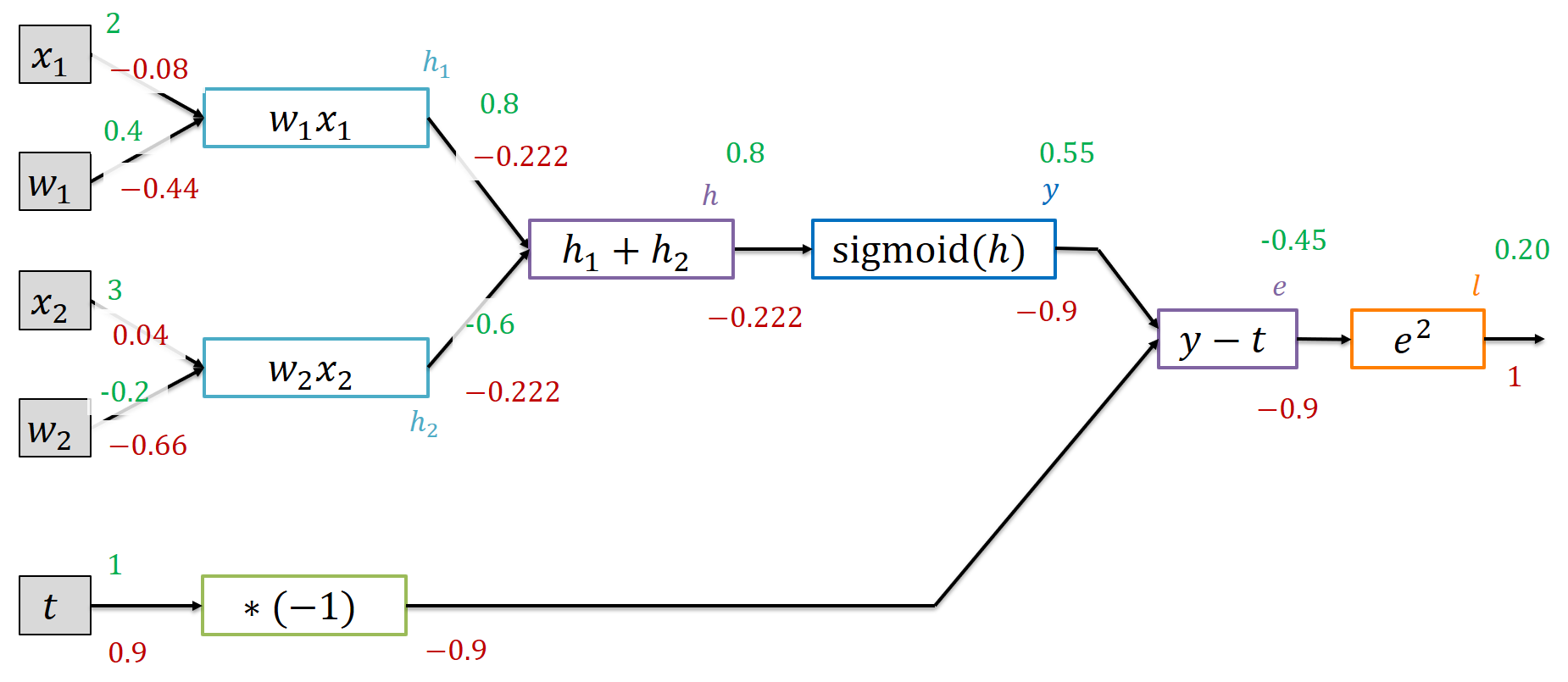
We also found gradients for the inputs that we cannot really change. It does not make sense to adapt the target $t$ to what would make the loss smaller (that’s a bit cheating !?), we need to change the output $y$. Similarly, we cannot change the inputs $\vec{x}$ (except for when we explicitly look for adversarial inputs that fool our network). But the weight gradients reveal some interesting aspects. The weight gradients are negative. That means that the loss is likely to go down if we increase the weight a little bit. And that makes perfect sense: we need to get $y$ higher, closer to 1. If we increase $w_1$, that will enforce the input $2$ and if we increase $w_2$, we perform a smaller subtraction - again leaving us with a higher value for $h$ and thus $y$.

The perspective of neural nets as that of multiple differentiable functions composed together is so prevalent that some people suggested to drop the term 'neural network' or even 'deep learning' in favor of differentiable programming.

Conclusion

Neural networks perform a calculation of a function composed of many simpler ones to transform an input into an output (e.g., a classification). During training, we need access to partial derivatives to perform parameter updates based on them. We can algorithmically calculate these derivatives and performed some experiments ourselves using a plain Python program. Finally, you have connected all necessary dots to proceed with actual implementations of automatic differentiation. Have fun!