Why so sigmoid??
TL;DR
We take a quick dive into why the sigmoid activation was so nice for early neural networks. Also, there is a neat derivation for its somewhat complicated arithmetic form (exponential in the denominator etc.).
Find a jupyter notebook accompanying the post here or directly in Colab:
|
|
Intuition of the sigmoid function
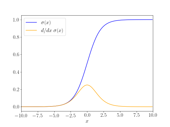
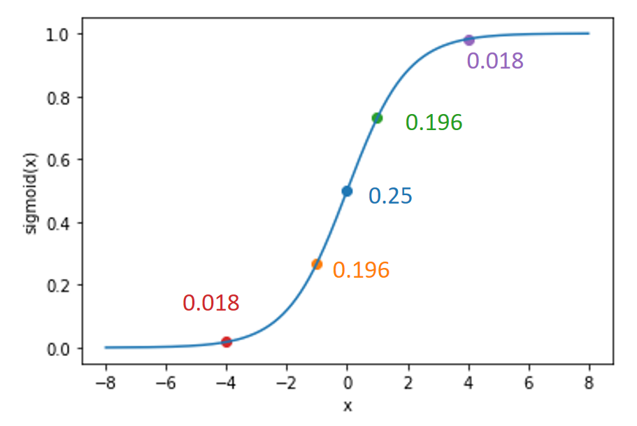
When you first learn about neural networks, it’s almost inevitable to encounter the sigmoid function
\[\sigma(x) = \frac{1}{1+e^{-x}}\]or its nicer graph:
The inputs to a neural network $(x_1, x_2, \ldots, x_m)$ are weighted with $(w_1, w_2, \ldots, w_m)$ and summed up to build an activation of a neuron. So far that seems reasonable. To calculate a score for a class “SPAM”, an occurrence of the word “Millions” might score high on the “spamness” scale (and be multiplied with a large weight) whereas “Dear Son” would reduce the “spamness” score (with a negative weight). But then that overall activation is fed to sigmoid, the activation function to form an output.
That’s it. That formula just appears out of the blue sky and is supposed to be the “right” choice. With exponential and everything. Why? Why that particular form and arithmetic? Is there something inherently special about it that we were just fortunate to discover?
Okay, we can also train with other functions. Still, sigmoid remains popular, especially for binary classification problems where the single output has to be a number between 0 and 1 to denote that probability of, say, class 1. When we consider the effect that weights $w$ and biases $b$ have on the shape of $\sigma(w \cdot x + b)$, we notice that sigmoid starts to resemble a step function:
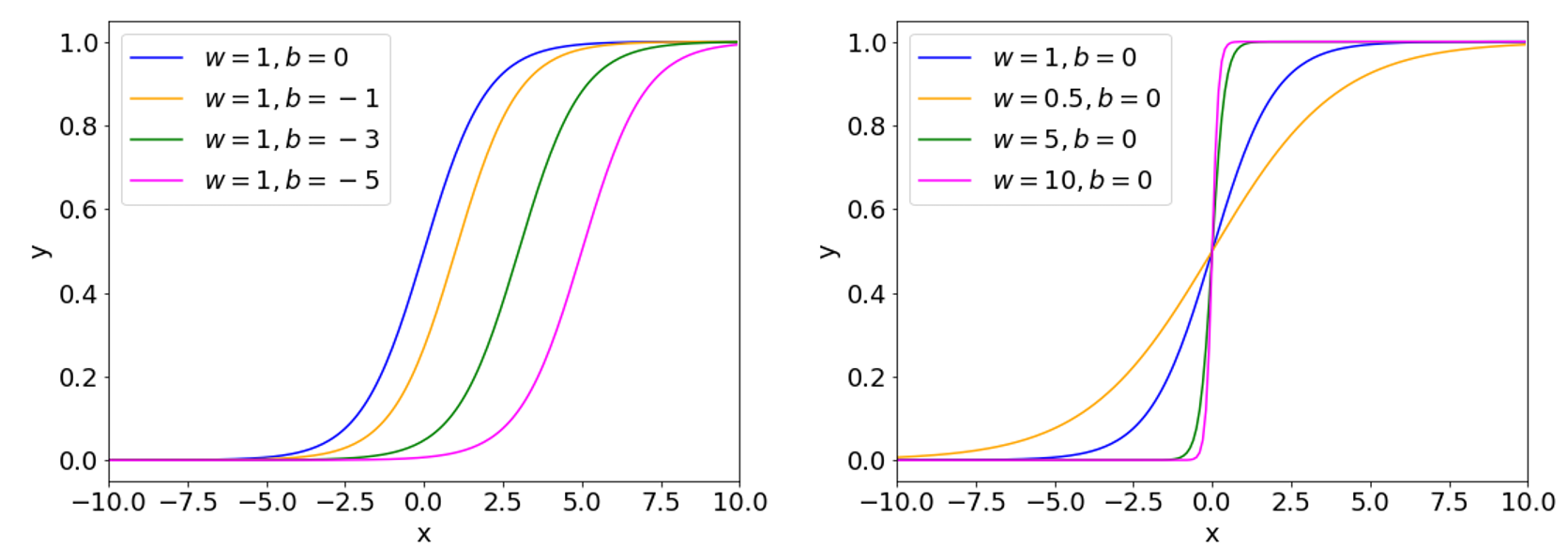
Now, step functions are much easier to conceptualize as a human. The sum of the weighted inputs must simply exceed a threshold (e.g., by setting a bias accordingly) for the activation to become positive and outputs 1, otherwise it returns 0.
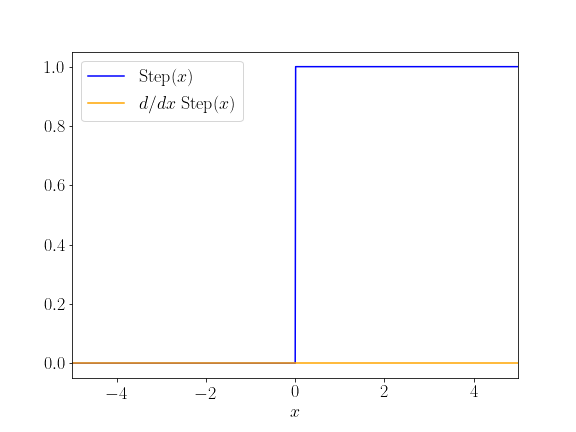
For a neural network they are a real nightmare, no non-zero gradient anywhere! But they greatly help us build intuition how a network might learn, as long as we replace a suitable sigmoid instance (that is differentiable) wherever we use steps. What do I really mean by that? Consider the following image, where we perform a weighted sum of pixel activation in a cartoon image to detect a vertical line on the right (which could be useful to identify a “4” or a “7” and separate it from an “8”):
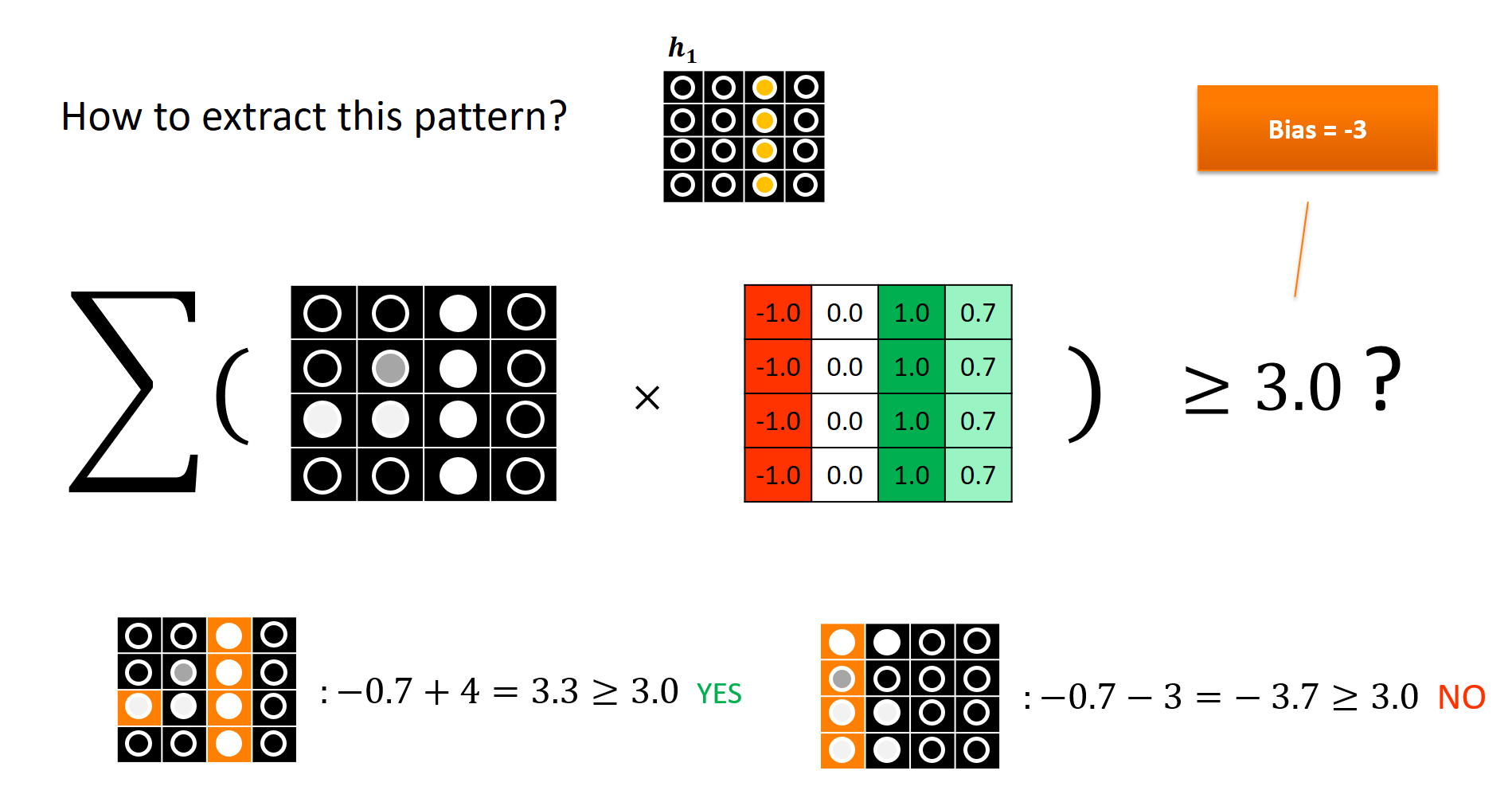
By setting a bias $b = -3$ and using the step function that outputs 1 only if its input is greater than 0, we get a “concept detector” that is active if enough positive evidence is collected for a certain pattern/concept. Here, that are all the inputs in the right region of an image to get a somewhat boolean concept “vertical line right” whose value ranges between 0 and 1. The orange cells indicate summands that are non-zero.
The key takeaway is that a neural network might discover similar weights and biases during training which makes the way sigmoids can be used more intuitive.
A probabilistic derivation of Sigmoid
It really bugged me that sigmoid came without any formal intuition as to its exact arithmetic form. Where does it come from? The deep learning book by Goodfellow, Bengio, and Courville offers some insight on page 179. But first let’s look at the “trick” that makes softmax successful in normalizing a finite set of scores (essentially we’ll be doing the same with sigmoid):
- Take unnormalized scores (they could be negative)
- Exponentiate them to make them positive (ha! that’s where the $e^x$ comes from)
- Sum all exponentiated values and normalize by that sum
That procedure will be guaranteed to produce $k$ values that sum to one and are all non-negative. You can safely interpret them as a probability mass function. Formally, we just derived the softmax function by assuming the unnormalized scores to be log-probabilities. For some reason I find that procedure easier to wrap my head around but now let’s go for sigmoid!
For sigmoid, we do just about the same for binary classification (classes 0 and 1), except that we fix the log-probability for event 0 to be 0 and place the log-probability for event 1 anywhere on the real line relative to that 0. Let’s walk through the calculations:
Note that these are two distinct cases (so normalization works only in isolation here). Let’s work out what happened here. Recall the first case:
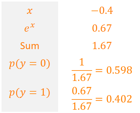
We started with the unnormalized log-probability for the event “1”. Let’s write that as $y = 1$ to make it a little prettier and call our score $x$ (here, -0.4). Hence we exponentiate and normalize to get the true probabilities:
\[\begin{align*} & \log \tilde{p}(y = 1) = x \\ & \log \tilde{p}(y = 0) = 0 \\ & \tilde{p}(y = 1) = e^x \\ & \tilde{p}(y = 0) = e^0 = 1 \Rightarrow \\ & p(y = 1) = \frac{\tilde{p}(y = 1)}{\tilde{p}(y = 0) + \tilde{p}(y = 1)} = \frac{e^x}{1 + e^x} = \frac{1}{e^{-x} + 1} = \frac{1}{1 + e^{-x}} \end{align*}\]where the last step involves dividing denominator and numerator by $e^x$.
Et voilà, we find that $p(y = 1) = \frac{1}{1 + e^{-x}} = \sigma(x)$ – the sigmoid function!
To convince yourself that this works, walk through the following code:
log_score1 = -0.4

# make exponentiating and normalizing explicit
score1 = np.exp(log_score1)
sum1 = score1+1
prob0 = 1 / sum1
prob1 = score1 / sum1
print(prob0, prob1)
>>> 0.598687660112452 0.401312339887548

# compare that to the output of sigmoid
# of the unnormalized score
print(1-sigmoid(log_score1), sigmoid(log_score1))
>>> 0.598687660112452 0.401312339887548
Derivative of Sigmoid
Besides emulating the functionality of a step function and acting as a binary “concept detector”, the sigmoid function is continuously differentiable over its whole input domain which is nice for gradient-based optimization. In particular, its derivative $\frac{d \sigma}{d x} $ is really easy to implement, once you know the value of $\sigma(x)$:
\[\frac{d \sigma}{d x} = \sigma(x) \cdot (1 - \sigma(x))\]You can read the derivation on Wikipedia. Let’s inspect the derivative at a couple of specific points:
The required code is pretty straightforward
def dsigmoid(x):
    return sigmoid(x) * (1.0 - sigmoid(x))

print(dsigmoid(-4))
>>> 0.017662706213291118
print(dsigmoid(1))
>>> 0.19661193324148185
and is validated by a simple gradient check (to see if we can trust the derivative):
def check_gradient(func, x):
    eps = 0.001
    numeric_gradient = (func(x+eps)-func(x)) / eps
    return numeric_gradient

print("Analytic gradient at 1:", dsigmoid(1))
print("Numeric gradient at 1:", check_gradient(sigmoid, 1))
>>> Analytic gradient at 1: 0.19661193324148185
>>> Numeric gradient at 1: 0.1965664984852067
Well, that looks good! It’s also due to this simple derivative that sigmoid used to be so popular for early neural networks. In fact, we can easily implement the local gradient of sigmoid in an autodiff framework such as the one described in this post.
class Sigmoid(CompNode):

    def __init__(self, x : CompNode, tape : Tape):
        self.x = x
        super().__init__(tape)

    def forward(self):
        self.output = 1. / (1. + np.exp(-self.x.output))

    # has to know how to locally differentiate sigmoid
	# (which is easy, given the output)
    # d sigmoid(x) / d x = sigmoid(x)*(1-sigmoid(x))
    def backward(self):
        local_gradient = self.output * (1. - self.output)
        self.x.add_gradient( local_gradient * self.gradient)
Universality of Sigmoid
Finally, sigmoid activations provide neural networks with a nice universal property: If we allow arbitrarily many hidden units, it can approximate functions up to a desired accuracy by building “tower functions” composed of two sigmoids.
I highly recommend Michael Nielen’s video or book explaining the universal approximation theorem (don’t worry, that sounds mathier than it is, at least to get the intuition).
In practice: Use Rectified Linear Units
Now, here comes the really anticlimactic part of this post … I’ve said so many nice things about sigmoid (probabilistic interpretation, nice derivatives, universal approximation) and yet, sigmoid activations are pretty much frowned upon nowadays in modern networks. Just head over to the TensorFlow playground to inspect the convergence behavior for sigmoid and ReLU. Why is that? Recall the first derivative of sigmoid:
It is very easy to have the network put in values in the saturated region of the function, i.e., where it asymptotes to 0 or 1. In these regions, there is very small derivative which leads to very slow (or even no) training.
The ReLU activation (= rectified linear unit) rightfully took its throne as the most popular activation function, starting from its birth roughly around the time AlexNet was published. ReLU is much simpler
\[\mathit{ReLU}(x) = \max (x, 0)\]Yeah, it’s just that. It cuts off the negative part and outputs the identity for the non-negative part.
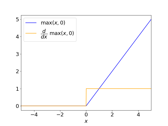
In the positive regime, the local gradient of ReLU is 1, everywhere. This is its big advantage over sigmoid. It basically “passes on” the gradient it receives to its input nodes in the computational graph. But you can maybe guess why people were reluctant to use ReLU functions … let’s address the elephant in the room: What happens at $x = 0$ to $\frac{\partial \mathit{ReLU} }{\partial x}$?

Mathematically speaking, the derivative is $0$ for $x < 0$ and $1$ for $x > 0$. It is not defined at $x = 0$. But that’s not really an issue in practice. In gradient-based training of neural networks, we essentially use the gradient as a mere guide to direct our weight updates. We don’t really need the precise derivative (this becomes even more apparent since we rarely use the pure gradient in optimization when we add momentum or normalizing squared gradients as in AdaGrad or Adam). Or, put more pragmatically, just use 1 or 0 for the derivative at $x = 0$. You’re very unlikely to hit that precise input during training, anyway.
For our autodiff framework, the implementation could look like this:
class ReLU(CompNode):

    def __init__(self, x : CompNode, tape : Tape):
        self.x = x
        super().__init__(tape)

    def forward(self):
        self.output = np.max( [self.x.output, 0])

    def backward(self):
        local_gradient = 1 if self.output > 0 else 0
        self.x.add_gradient( local_gradient * self.gradient)
The gradient is defined for two cases but since we’re always asking for concrete values (e.g. of our weights) this constiutes no big problem.
Finally, why should you still know about sigmoid if there are much fancier activation functions out there?
For once, sigmoid is still safe to use as an output node for binary classification where you just need to get a value between 0 and 1. In the output layer, usually enough gradient stays “alive” for the hidden layers. Other than that, it’s still used in many introductory texts and makes the presentation of local gradients easier to explain. And its fancier cousin, tanh, which provides both negative and positive output values is still widely used in recurrent neural networks, such as LSTMs.
Conclusion
Sigmoid is often taken for granted. It is treated simply as a continous, differentiable approximation to a step function that produces a value between 0 and 1. That’s less than it deserves. If we interpret an output score as an unnormalized log-probability, it emerges quite naturally from exponentiating and normalizing. And it has a very convenient derivative. While not showing the best gradient properties for hidden units in practice, it remains still relevant as output activation* for binary classification tasks.