A worked example of backpropagation

TL;DR

Backpropagation is at the core of every deep learning system. CS231n and 3Blue1Brown do a really fine job explaining the basics but maybe you still feel a bit shaky when it comes to implementing backprop. Inspired by Matt Mazur, we’ll work through every calculation step for a super-small neural network with 2 inputs, 2 hidden units, and 2 outputs. Instead of telling you “just take the derivatives and update the weights”, we’ll take a more direct approach and work out the ideas by inspecting what the network would be doing, without any calculus or linear algebra. We will then add the matrix magic to make our code nice and tidy. And you get to implement a single backprop step only in Numpy – without too much headache! Let’s connect the dots!

If you already know backpropagation, gradient descent etc. and just want to see the toy example, click here. Otherwise, grab a pencil and enjoy the ride!

Find a jupyter notebook accompanying the post here or directly in Colab:

Run in Google Colab

Backpropagation by intuition (without the calculus stuff)

Backpropagation is the algorithm that runs deep learning. Approaching it for the first time might however feel daunting. You will read about backpropagation of the error, reverse-mode autodiff, calculus, Jacobian, delta-rule … and either stick with “well, I don’t care, TensorFlow/PyTorch/<insert other fancy DL framework> will do the job” or spending a generous amount of paper deriving equations by hand. I think neither is really necessary. It’s best to see the calculations in action and implement them by yourself.

Why should you even care? As Andrej Karpathy put it, backprop is a leaky abstraction, meaning that you sometimes need to get your hands dirty debugging problems with backprop and not treat it as a black box. Therefore it helps to understand the dynamics of how a neural network is actually trained.

In a nutshell, backpropagation is the algorithm to train a neural network to transform outputs that are close to those given by the training set. It consists of:

• Calculating outputs based on inputs (features) and a set of weights (the “forward pass”)
• Comparing these outputs to the target values via a loss function
• Calculating “weight change requests” aka gradients to reduce the loss (the “backward pass”)
• Increasing/decreasing the weights according to the gradients (the “gradient descent” step)

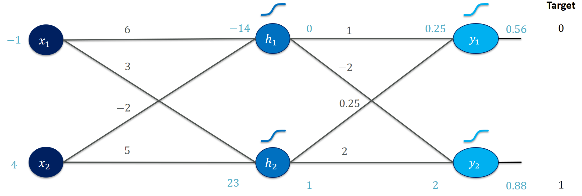
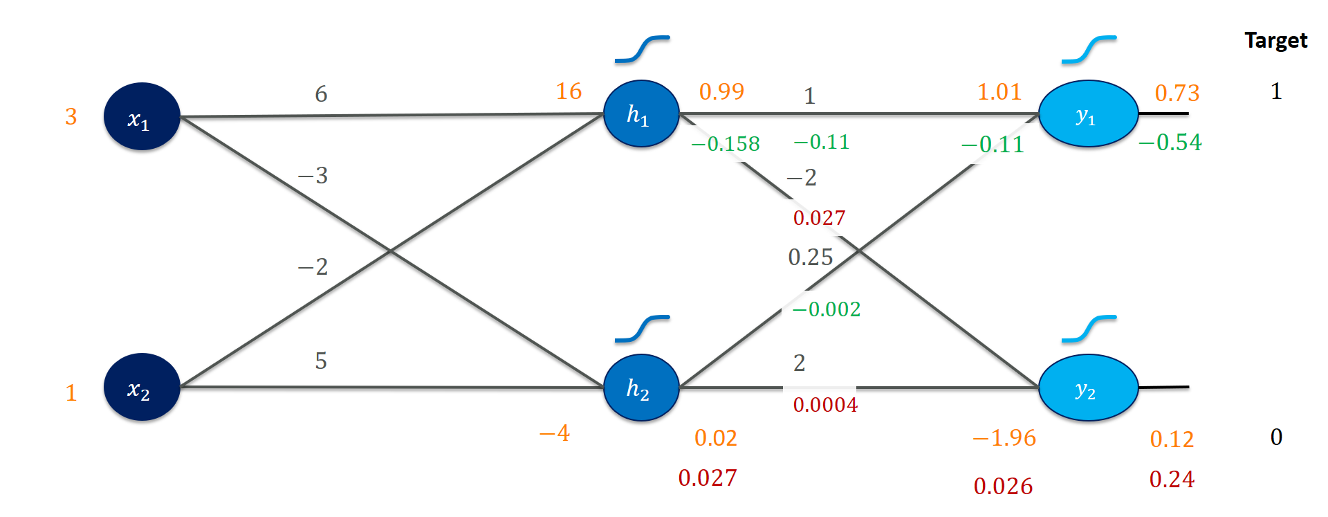
We will work through all of them using a toy network we are going to play with:

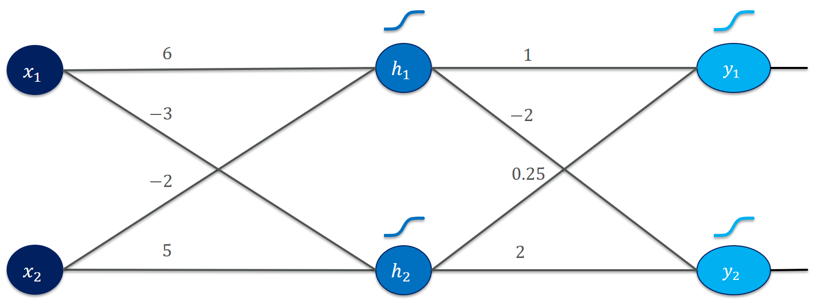
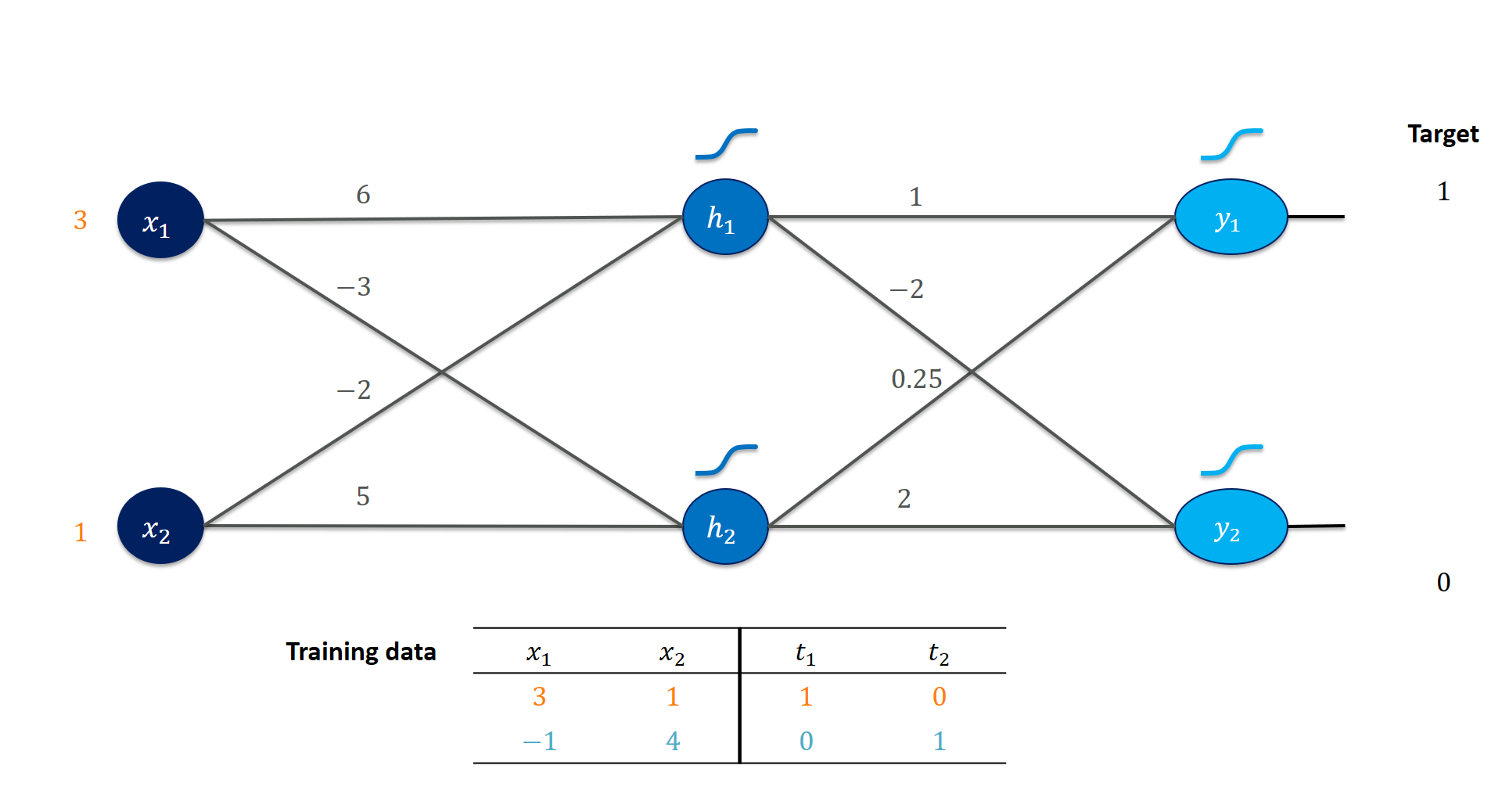
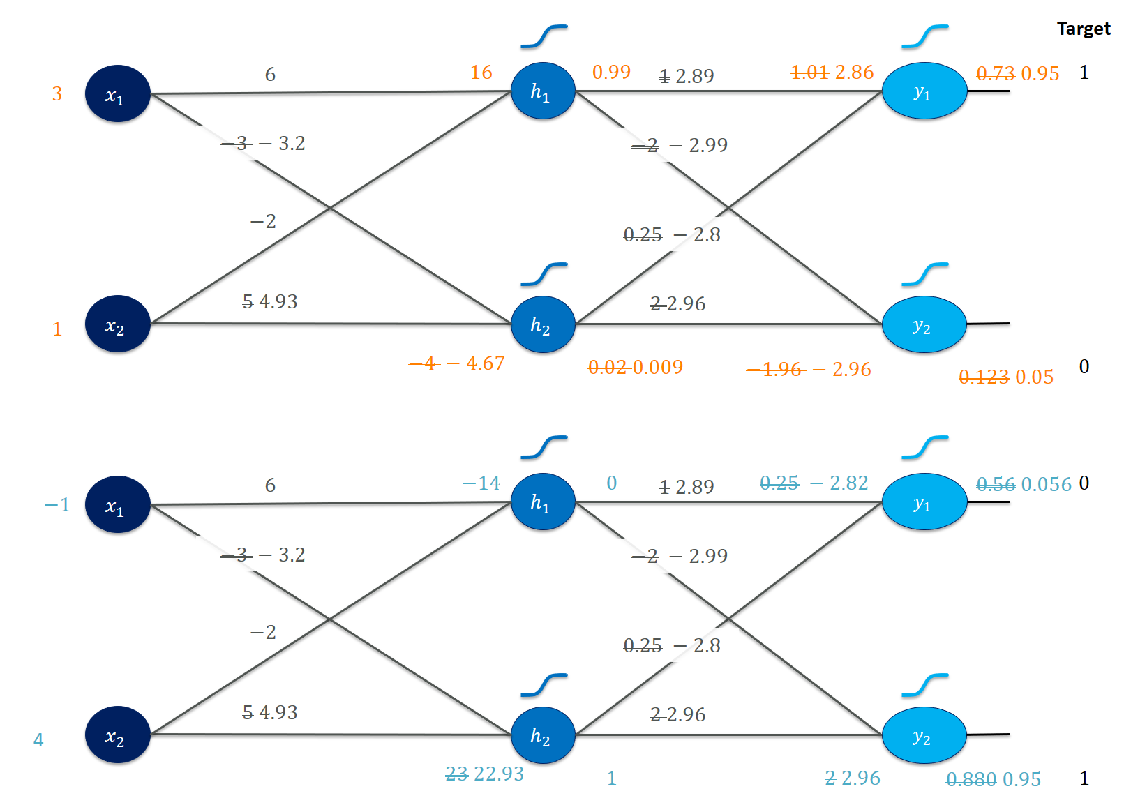
I actually suggest scribbling it on paper or leaving it aside on a separate monitor to have it handily available. It is a simple feedforward network (used to be called “multilayer perceptron”, MLP) that consists of two inputs ($x_1$ and $x_2$), two hidden units ($h_1$ and $h_2$) and two outputs ($y_1$ and $y_2$). The weights (6, -3, etc.) specify how to multiply together the input values to form a hidden activation and, finally, an output. For the moment, we ignore biases to keep things simple. We use the (almost infamous nowadays) sigmoid activation function for both the hidden units and the output units. Our training set is equally simple:

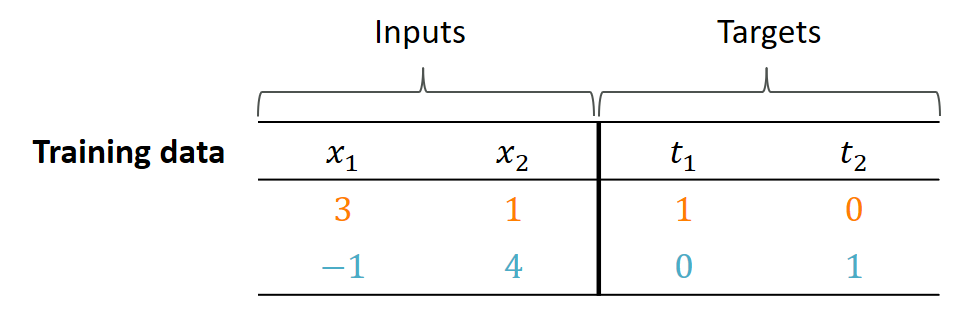
When presented with inputs $(3, 1)$, our network should output the target values $(1, 0)$ for $(y_1, y_2)$. Think of the outputs as classes such as cat or dog. For $(-1, 4)$ it should output $(0, 1)$. How well is our network doing with its current weights?

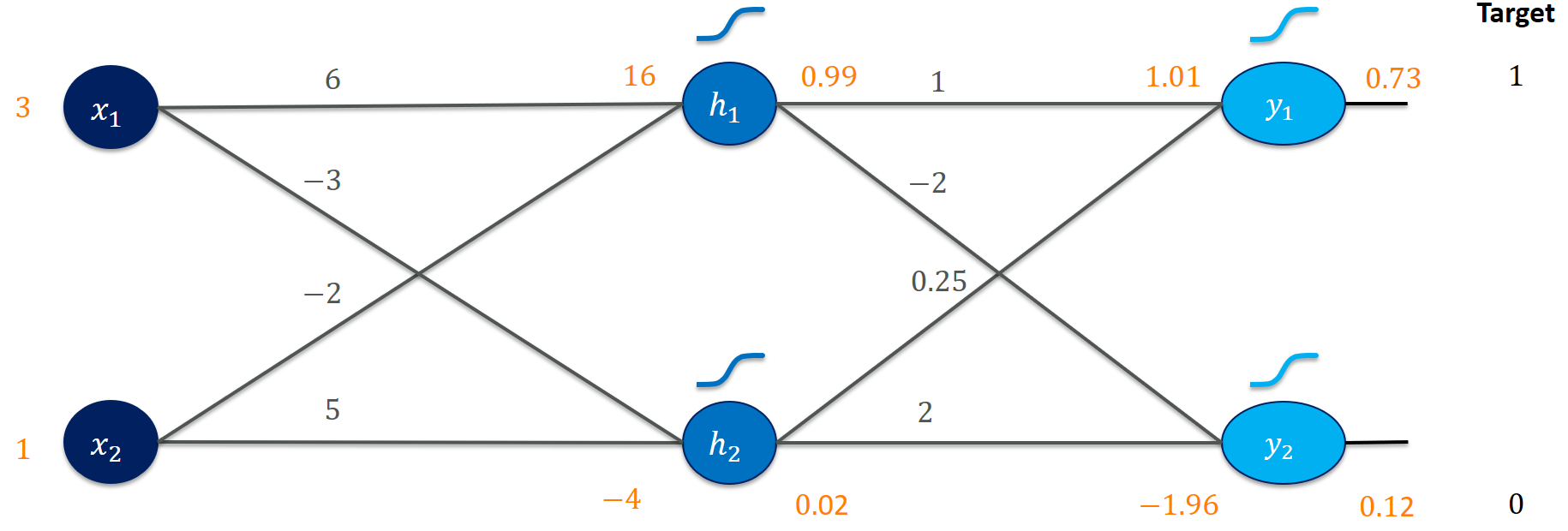
It’s actually not terribly far off! The output $y_1 = 0.73$ is somewhat close to 1 and the output $y_2 = 0.12$ is close to 0. Certainly, both could be closer to the target values. But what did we exactly calculate?

First, we get the activation as the weighted sum of inputs for each neuron. Let’s do this for $h_1$:

x1, x2 = 3., 1.
h1_in = 6*x1 + (- 2)*x2 
>>> 16.0

Next, we feed this information through the activation function (as we mentioned, sigmoid):

def sigmoid(z):
    return 1./(1+np.exp(-z))
h1_out = sigmoid(h1_in)
>>> 0.9999998874648379

When first encountering sigmoid activations, I was pretty terrified. Why do we exactly pick that function and what’s with all those weird exponentials in the denominator? It’s perfectly fine to think of sigmoid just as a possibility to implement a (smooth) ‘switch’ that can be on or off. I dedicated another post to sigmoid.

We perform exactly the same calculations (with the respective weights) for h2_in, h2_out, y1_in, y1_out, y2_in, and y2_out:

y1_in = 1*h1_out + 0.25*h2_out
y1_out = sigmoid(y1_in)

y2_in = (-2)*h1_out + 2*h2_out
y2_out = sigmoid(y2_in)

This will give us, for example, y1_out = 0.7319. All these calculations are called the forward pass of a neural network. Fair enough.

Changing weights to improve our neural network

Here the central question arises:

How should I change the weights to improve my outputs?

As an analogy, think of how you would turn the knobs in a shower to achieve the desired target temperature? If it is too cold, increase the warm water and decrease the warm water; If it is too hot, do the converse.

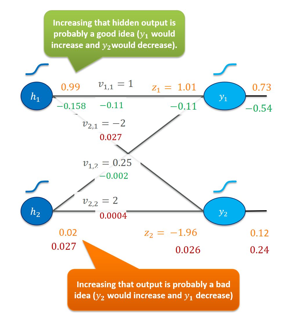
Let’s zoom in on the last layer first:

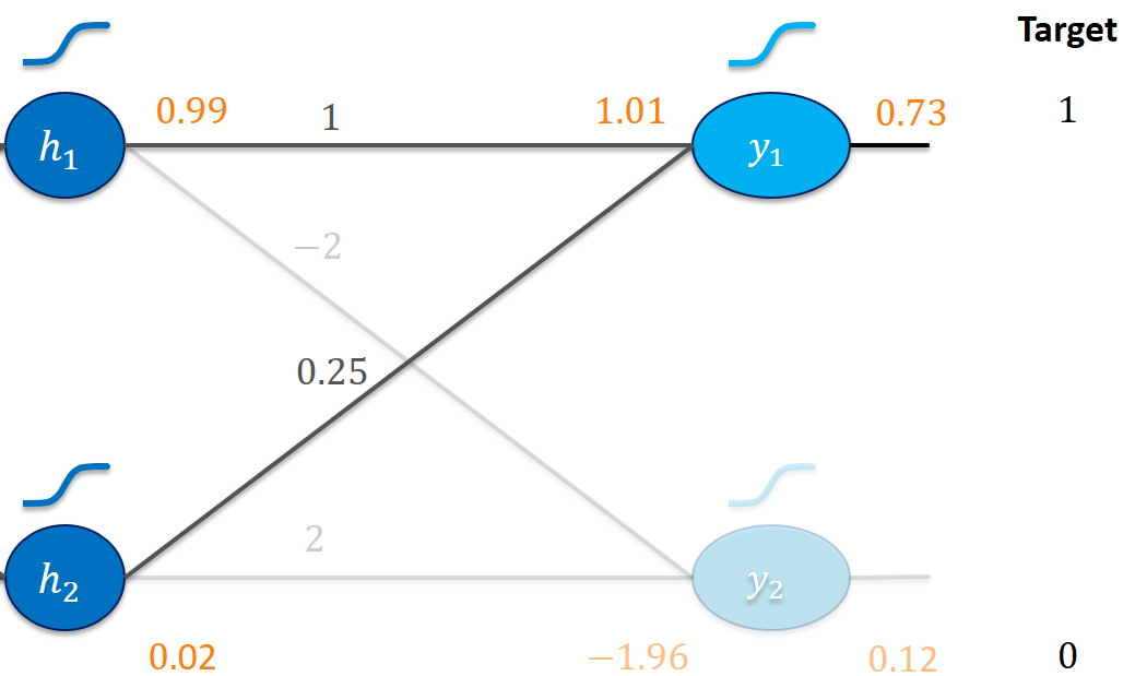
Our goal is clearly to make y1_out larger and y2_out smaller. Increasing the weight 1 (e.g., use 1.01 instead) seems like a good idea here. It would be multiplied with the 0.99 from h1_out and immediately lead to a higher activation y1_in (and thus y1_out). Increasing 1 is probably also more effective than increasing 0.25 to get us to a higher y1_in since a change in 0.25 gets multiplied by the much smaller h2_out = 0.02. We would probably have to make much more of an effort (increasing 0.25) to get us somewhere close to y1_out = 1.

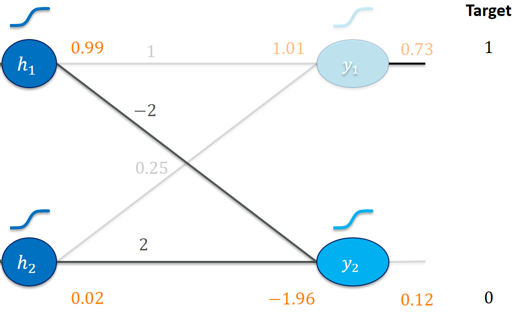
Here, increasing -2 (to, say, -1.9) would be a bad idea since that would make y2_in (and y2_out) greater! A smaller weight of -2.01 would probably make things better. Similarly, we would reason to decrease the weight 2.

But the weights (of that layer) are, of course, not the only way to manipulate the output values. Indirectly, the weights of the first layer affect the values for h1_out and h2_out. Note how increasing h1_out would be a great idea for both outputs: y1_out would get larger (due to the weight 1) and y2_out would get smaller (due to the weight -2).

This is where backpropagation steps in: similar to how we worked out how to manipulate the weights in the last layer if we want to increase $y_1$ and decrease $y_2$, we could figure out how to manipulate the weights in the first layer to make $h_1$ larger (and perhaps $h_2$ smaller for $y_2$). That is why people call it backpropagation of the error since our goal is to make the error (difference between current output and target) small and this works by finding out how to tweak the weights back in previous layers.

But wait, we just focused on our first training instance? Here’s the forward pass for the second example (verify that you understand how these values emerge):

The network does significantly worse on this instance and needs more adjusting to come closer to the target values. Which weights would you adjust (and how) to improve the performance? To calculate the forward pass in one go, here is a handy (explizit) method that expects the weights as a list of values, e.g., [6, -3, -2, 5, 1, -2, 0.25, 2].

def forward(x, w):
    h1_in = x[0] * w[0] + x[1] * w[2]
    h2_in = x[0] * w[1] + x[1] * w[3]
    
    h1_out = sigmoid(h1_in)
    h2_out = sigmoid(h2_in)
    
    y1_in = h1_out * w[4] + h2_out * w[6]
    y2_in = h1_out * w[5] + h2_out * w[7]
    
    y1_out = sigmoid(y1_in)
    y2_out = sigmoid(y2_in)
    return y1_out, y2_out

Backpropagation (with the calculus stuff)

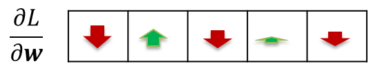
So far, we have only gained a very vague idea about how to adjust our weights.

• “Increasing that weight (1) might be a good idea.”
• “Increasing that weight (-2) might be a bad idea.”
• “Increasing that weight (1) is probably going to have a stronger effect than that weight (0.25).”

It’s now time to make these statements more precise such that we can implement them in our training algorithm. It’s still helpful to keep those intuitions in mind because that is how we should think of “weight change requests”. This is where calculus steps in to derive the necessary expressions.

Loss functions

Instead of saying “our outputs should be close to the targets”, we specify a scalar loss function $L$ (i.e., a number) that does just that. It judges a vector of weights $\vec{w}$ such as $(6, -3, -2, 5, 1, -2, 0.25, 2)$ by its performance to meet the target values. A bad performance will yield a high loss, a good performance will yield a low loss. We then take derivatives of the loss with respect to each one of the weights individually to see how increasing that particular weight would probably affect the loss. These values will become our “weight change requests” … but we’re getting ahead of ourselves.

Typical loss functions include (mean) squared errors or the cross-entropy between output and target. For our problem, we chose a particularly simple loss function, the sum of squared errors. It compares every output $y_i$ with a target $t_i$ and sums up the squared differences:

\[L(\vec{w}) = (y_1 - t_1)^2 + (y_2 - t_2)^2\]

Since $x_1$ and $x_2$ as well as $t_1$ and $t_2$ are given by training set, the $L$ only depends on the weights $\vec{w}$. The loss would achieve its minimal value 0 if every output is exactly equal to the target values. Every deviation (e.g., 0.73 instead of 1) is punished proportionally to the size of the error. What would be the loss for our current network with $\vec{w} = (6, -3, -2, 5, 1, -2, 0.25, 2)$?

sq_err1 = (y1_out - 1)**2 
sq_err2 = (y2_out - 0)**2
sse = sq_err1+sq_err2
>>> 0.08699208259994781

which is just the loss for the first training instance (what is it for the second one?).

You can verify for yourself that a network with weights $\vec{w} = (6, -3, -2, 5, \mathbf{2}, \mathbf{-2.5}, \mathbf{0.3}, \mathbf{1.5})$ - which is tweaked according to our intuition from above - would yield better results on the first training instance:

print(y1_out, y2_out)
>>> 0.8813624223958589 0.07777132641389171

and that would also be reflected in a lower loss:

print(sse)
>>> 0.020123254031954686

Now it’s time to figure out how we can systematically move from the first to the second set of weights in order to get to networks with a very low loss function value.

Why do we even care for loss functions for a classifier if we are just interested in the one with the highest accuracy? Loss functions differ from performance measures (sometimes simply called metrics) such as accuracy, precision, or recall (that we actually care to optimize) in that they are differentiable and therefore suitable for gradient-based learning. Our hope is that a good set of weights according to the loss is also a great choice for our ultimate goal.

Using derivatives to adapt weights

Let’s start off really easy and consider a 1D case. Our prediction is a function $y = w \cdot x$ and $y$, $w$, and $x$ are just real numbers (scalars). Let’s say we have currently set $w = 3$ and have a training instance $(x, t) = (4, 8)$. Our output would then be $12$ and the loss would be:

\[\begin{align*} L(w) &= (y - t)^2 = (x\cdot w - t)^2 \\ L(3) &= (12 - 8)^2 = 16 \end{align*}\]

Since we have access to the loss function $L(w)$ for every point on the real line, we could try to see what happens if we increase $w$ just a tiny little bit ($\Delta = 0.01$):

\(L(3.01) = (12.04 - 8)^2 = 16.32\) The loss also increased, so it’s a bad idea to increase $w$. In fact, for a $0.01$ increase in $w$, we incurred a $0.32$ increase in the loss! This ratio of loss after/before increasing $w$ starts to look familiar to a difference quotient:

\[\frac{16.32 - 16.0}{3.01 - 3.0} = \frac{L(w + \Delta) - L(w)}{\Delta}\]

We would rather decrease $w$ to, say, 2.99!

Conversely, if we started with $w = 1.5$, our output would be $y = 1.5\cdot 4 = 6$ and

\[\begin{align*} L(1.5) &= (6 - 8)^2 = 4 \\ L(1.51) &= (6.04 - 8)^2 = 3.84 \end{align*}\]

So, a tiny increase in $w$ made the loss go down - we would increase $w$ now. The fraction between change in loss to change in $w$ now boils down to $\frac{-0.16}{0.01}$, i.e., $-16$, a negative value.

At this point you might either be wondering how to come up with the tiny small step $\Delta$ or you know where this journey is headed. By letting $\Delta$ go to 0, we can find the limit value of that loss change ratio, i.e., we differentiate the loss function with respect to $w$. This will give us a value we can precisely calculate that captures the effect a small increase on $w$ has on the loss value $L(w)$. If this seems confusing, I wholeheartedly recommend watching this video by 3Blue1Brown.

\[\lim_{\Delta \to 0} \frac{L(w + \Delta) - L(w)}{\Delta} = \frac{d L(w)}{d w}\]

We can use the first derivative of $L$ as a guide for how to update $w$. And, we can precisely calculate that value for any concrete $w$! Let’s do this manually for our example:

\[\begin{align*} &L(w) = (y - t)^2 = (xw - t)^2 = x^2 w^2 - 2 xwt + t^2 \\ &\frac{d }{d w} x^2 w^2 - 2 xwt + t^2 = 2 wx^2 - 2xt = 2x (wx - t) = 2x \underbrace{(y -t)}_{e} \end{align*}\]

Let’s check that this expression works properly:

def dLoss(w, x, t):
    return 2*x*(w*x-t)

print (dLoss(3., 4., 8.))
>>> 32.0
print (dLoss(1.5, 4., 8.))
>>> -16.0

which fits to what we observed with small 0.01 steps. Using the derivative in that fashion gives us a neat update rule for weights:

• If $\frac{d L }{d w} > 0$ then decrease the weight $w$ (loss is rising when increasing $w$)
• If $\frac{d L }{d w} < 0$ then increase the weight $w$ (loss is falling when increasing $w$)

But wait, why did I write $\frac{\partial L}{\partial w} L$ instead of $\frac{d L}{d w}$? Usually, we just have way more than one weight $w$ to optimize, for example if we had an offset parameter $y = w_0 + w_1 \cdot x$. Then our loss depends on both weights $L(w_0, w_1)$, simply written as $L(\vec{w})$. Mathematicians use the symbol $\partial$ to distinguish a partial derivative from $d$ for “normal” derivatives. This simply means that a function depends on multiple variables (e.g., $f(x,y,z)$) and we make it explicit what variable we are differentiating. For example:

\[\begin{align*} f(x,y) &= 3x^2 + 2xy + 5 \\ \frac{\partial f}{\partial x} &= 6x + 2y \\ \frac{\partial f}{\partial y} &= 2x \end{align*}\]

When we collect all partial derivatives in a vector (for convenience), this vector is called the gradient and is written as $\nabla$:

\[\begin{align*} f(x,y) &= 3x^2 + 2xy + 5 \\ \nabla f &= \begin{bmatrix} \frac{\partial f}{\partial x} \\ \frac{\partial f}{\partial y} \end{bmatrix} = \begin{bmatrix} 6x + 2y \\ 2x \end{bmatrix} \end{align*}\]

This gradient is defined as a function of $x$ and $y$ and could now be evaluated at any specific point. Let’s try this with $x = 2$ and $y = 3$:

def f(x,y):
    return 3*x**2 + 2*x*y + 5

def df_dx(x,y):
    return 6*x + 2*y

def df_dy(x,y):
    return 2*x

print(f(2, 3))
>>> 29
print(df_dx(2, 3))
>>> 18
print(df_dy(2, 3))
>>> 4

Phew, now that escalated quickly. Let’s just recap what we did here and why. For our loss function, we use a derivative for a single weight to find out whether to increase or decrease it. Since we have to do this for a bunch of weights (and not a single one), we need to collect all partial derivatives to form the gradient. I still visualize the gradient as a vector of “weight change requests” along the lines of “make $w_1$ much larger, make $w_2$ a bit smaller, make $w_3$ a bit larger, …”.

Backprop for the sample network

At this point of learning backprop, I was severely nervous about taking all those derivatives by hand … Fortunately, this tedious procedure is a mechanical operation that we can quite easily automate. I dedicated another post to the basics of it.

I assume our forward pass took place according to this code:

x1, x2 = 3., 1.
w11, w21 = 6., -2.
w12, w22 = -3., 5.

h1_in = w11*x1 + w21*x2
h2_in = w12*x1 + w22*x2
h1_out, h2_out = sigmoid(h1_in), sigmoid(h2_in)

# next layer 
v11, v21 = 1., 0.25
v12, v22 = -2., 2
y1_in = v11*h1_out + v21*h2_out
y2_in = v12*h1_out + v22*h2_out

y1_out, y2_out = sigmoid(y1_in), sigmoid(y2_in)

Backpropagation essentially consists of calculating the partial derivatives (the gradient) and adapting the weights according the gradient descent idea. We’ll walk through the backward calculations for the gradient of our network in three ways:

1. Manual calculation of every needed partial derivative

2. Algorithmic calculation using an autodiff system

3. Vectorized implementation using matrices

I want to emphasize that essentially all ways lead to Rome, i.e., they’re doing the same work. There are no shortcuts. Unless we’re factoring in the optimized hardware implementations (e.g., GPUs or distributed execution), the approaches are algorithmically equivalent.

To follow along, it really pays off to revisit the chain rule (again, 3Blue1Brown saves the day!).

Here's a very cheap analogy to the chain rule. Suppose you drive a car at 60 km/h. Depressing the accelerator pedal just a little (say 0.01 mm) leads to an increase of 0.5 km/h. Every increase of 0.01 km/h in speed leads to an increase of 0.03 g CO2. How much CO2 increase does the pedal depression of 0.01 mm cause? Well, just multiply 0.03 * 0.5 = 0.015.

Once we’re done with calculating the gradients, we’ll inspect how a weight update affects the accuracy of our network.

Manual calculation of every needed partial derivative

Alright, it’s time to work out every partial derivative. We begin with the first training instance. Let’s first outline what we are about to do: We’ll start differentiating the loss function with respect to its inputs. There are some partial derivatives (I call them “gradients”, in accordance with most of the community) that we really care about (those regarding parameters) and some that we need in order to calculate the former.

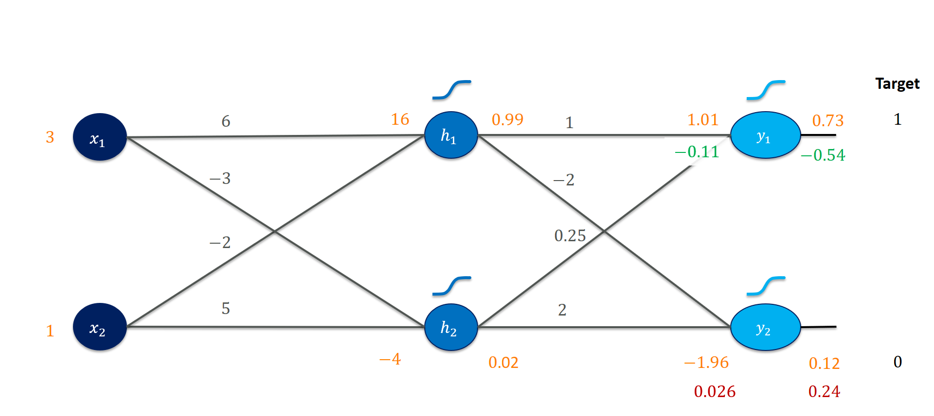
Let’s zoom in on the output, the last layer that produced the loss value:

Here, our question begins with the gradients for $y_1$ and $y_2$. How would increasing them affect the loss? Since 0.73 should be closer to 1 and 0.12 be closer to 0, we’d expect the gradient of $y_1$ to be negative (the loss goes down) and the gradient of $y_2$ to be positive (making $y_2$ larger would also make the loss larger). And that is exactly what we observe.

We get

\[\begin{align*} & L(y_1, y_2) = (y_1 - t_1)^2 + (y_2 - t_2)^2 = e_1^2 + e_2^2 \\ & \frac{\partial L}{\partial y_1} = \underbrace{2 \cdot e_1}_{\Large \frac{\partial L}{\partial e_1}} \cdot \underbrace{1}_{\Large \frac{\partial e_1}{\partial y_1}} + \underbrace{0}_{ \Large \frac{\partial e_2}{\partial y_1} } = 2e_1 \\ \end{align*}\]

In code:

t1, t2 = 1., 0.
e1, e2 = (y1_out-t1), (y2_out-t2)
print(e1, e2)
>>> -0.2680582866305111 0.12303185591001443

grad_y1_out = 2*e1
grad_y2_out = 2*e2
print(grad_y1_out, grad_y2_out)
>>> -0.5361165732610222 0.24606371182002887

To get the value before the sigmoid activation function is now rather straightforward, due to the nice derivative of sigmoid: Given $z$ and $\sigma(z) = (1 + e^{-z})^{-1}$:

\[\frac{\partial \sigma}{\partial z} = \sigma(z) \cdot (1 - \sigma(z))\]

Using that local derivative, we can simply apply the chain rule twice:

# backprop through sigmoid, simply multiply by sigmoid(z) * (1-sigmoid(z))
grad_y1_in = (y1_out * (1-y1_out)) * grad_y1_out
grad_y2_in = (y2_out * (1-y2_out)) * grad_y2_out
print(grad_y1_in, grad_y2_in)
>>> -0.10518770232556676 0.026549048699963138

This is fairly comfortable since we stored the outputs of the sigmoids, y1_out and y2_out. That leaves us with the following intermediate state after the output layer.

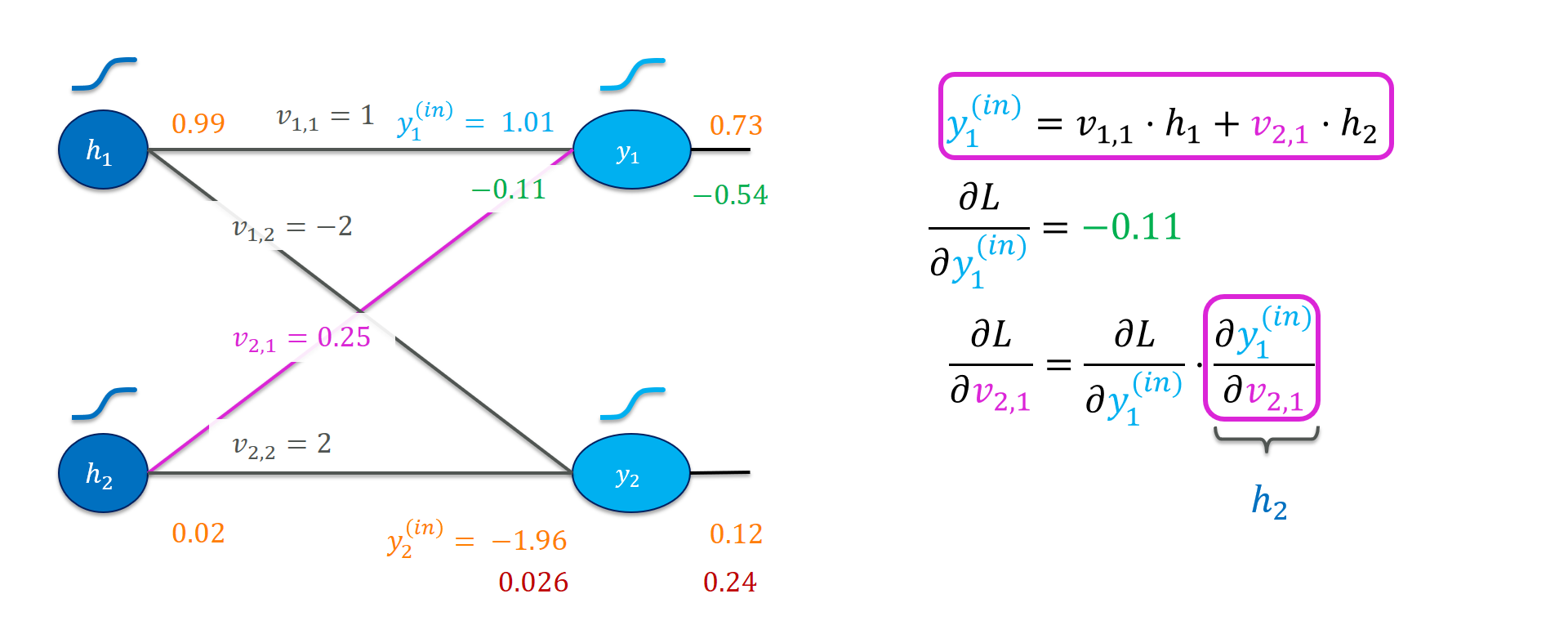
Next, we’re going after the first set of weights! Consider the weight $v_{2,1}$. It connects the output of the second hidden unit $h_2$ to the output $y_1$. That is its only effect on the loss function. We already know the loss gradient for $y^{(\mathit{in})}_1$, so we only need to add in the effect increasing $h_2$ has on it (by applying the chain rule appropriately).

Analogously, we can derive the gradients for all of the $v_{i,j}$ weights.

grad_v21 = grad_y1_in * h2_out
grad_v22 = grad_y2_in * h2_out 
print(grad_v21, grad_v22)
>>> -0.0018919280994576303 0.0004775167642113309

grad_v11 = grad_y1_in * h1_out
grad_v12 = grad_y2_in * h1_out 
print(grad_v11, grad_v12)
>>> -0.10518769048825163 0.02654904571226164

That’s great, we now know four of the eight gradients we’re after! But so far, the calculations match those of logistic regression (linear regression with a sigmoid output). How to proceed to the earlier layer? It is actually quite straightforward: we work out the gradients for the hidden units $h_1$ and $h_2$ and treat them as if they were output units. For example, finding that the gradient for $h_1$ were positive would lead to an incentive in decreasing that hidden activation – just as we had an incentive to decrease $y_2$ towards 0. From there, the calculations will be analogous to what we’ve already seen.

Let’s see this in action for the hidden unit $h_1$:

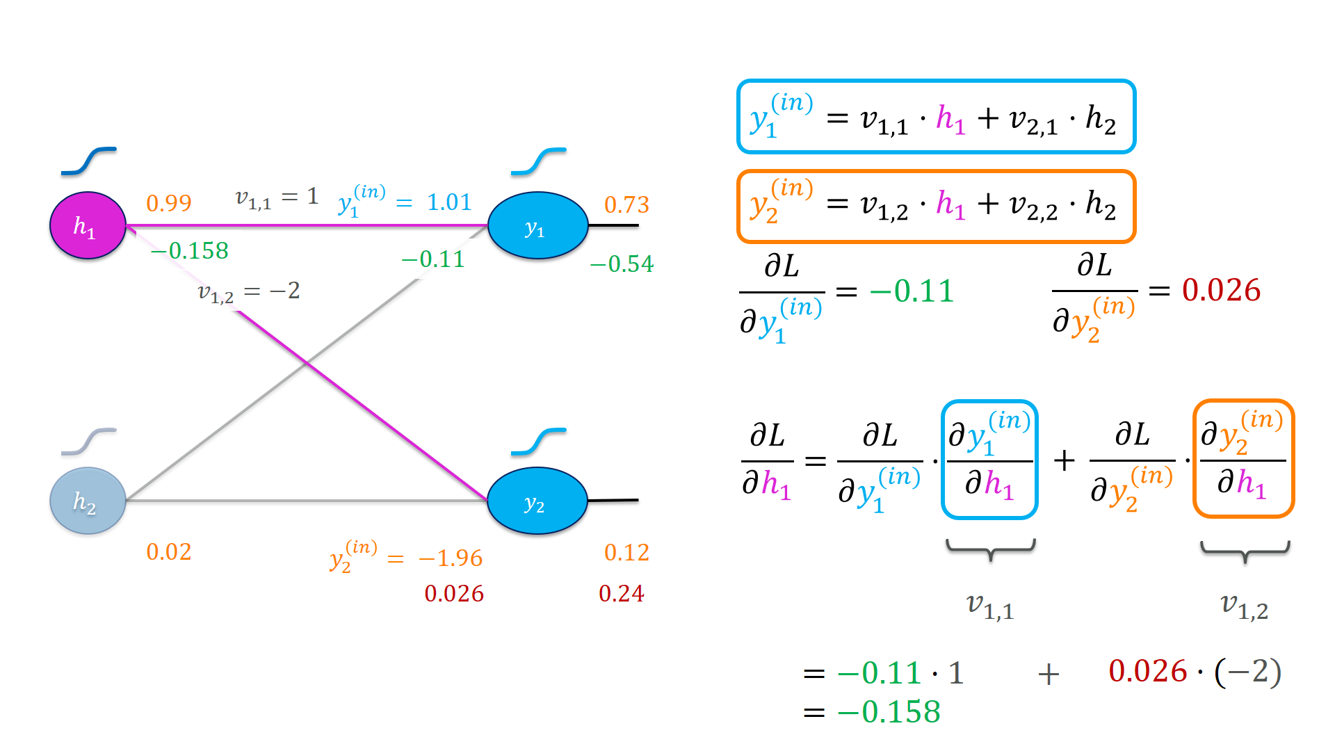
Notice how the output of $h_1$ affects the loss function on two paths, for the first time. Once via $y_1$ and once via $y_2$. Both are affected if we increase $h_1$ and we need to sum up these effects. An interesting pattern emerges here: The backward pass to the hidden activation looks similar to the forward pass. We take a weighted sum of the gradients of the outgoing nodes of the hidden activation.

grad_h1_out = grad_y1_in*v11 + grad_y2_in*v12
grad_h2_out = grad_y1_in*v21 + grad_y2_in*v22
print(grad_h1_out, grad_h2_out)
>>> -0.15828579972549303 0.026801171818534586

At this point, we are done with the output layer and its weights. Backpropagation of the error has happened since we now have gradients for the hidden activations that play a role similar to the output units. I think it’s very useful to play with the gradients we have so far:

Our wish that $h_1$ should be increased is a job that the weights of the previous layer have to take care of. Perform similar thought experiments for the weights. Do the gradients make sense to you?

From here on, it is pretty straightforward since we simply walk through exactly the same calculations again: Go back through the hidden activation, find the weight gradients, and get the gradients for the previous activation. Since that activation is already the input, we wouldn’t really need a gradient for $x_1$ (it doesn’t hurt to calculate it, though).

# backprop through sigmoid, simply multiply by sigmoid(z) * (1-sigmoid(z))
grad_h1_in = (h1_out * (1-h1_out)) * grad_h1_out
grad_h2_in = (h2_out * (1-h2_out)) * grad_h2_out

# get the gradients for the weights
grad_w21 = grad_h1_in * x2
grad_w22 = grad_h2_in * x2 

grad_w11 = grad_h1_in * x1
grad_w12 = grad_h2_in * x1 

# get the gradients for the inputs (could be ignored in this case)
grad_x1 = grad_h1_in*w11 + grad_h2_in*w12
grad_x2 = grad_h1_in*w21 + grad_h2_in*w22

This will give us the final gradient picture for the first training instance:

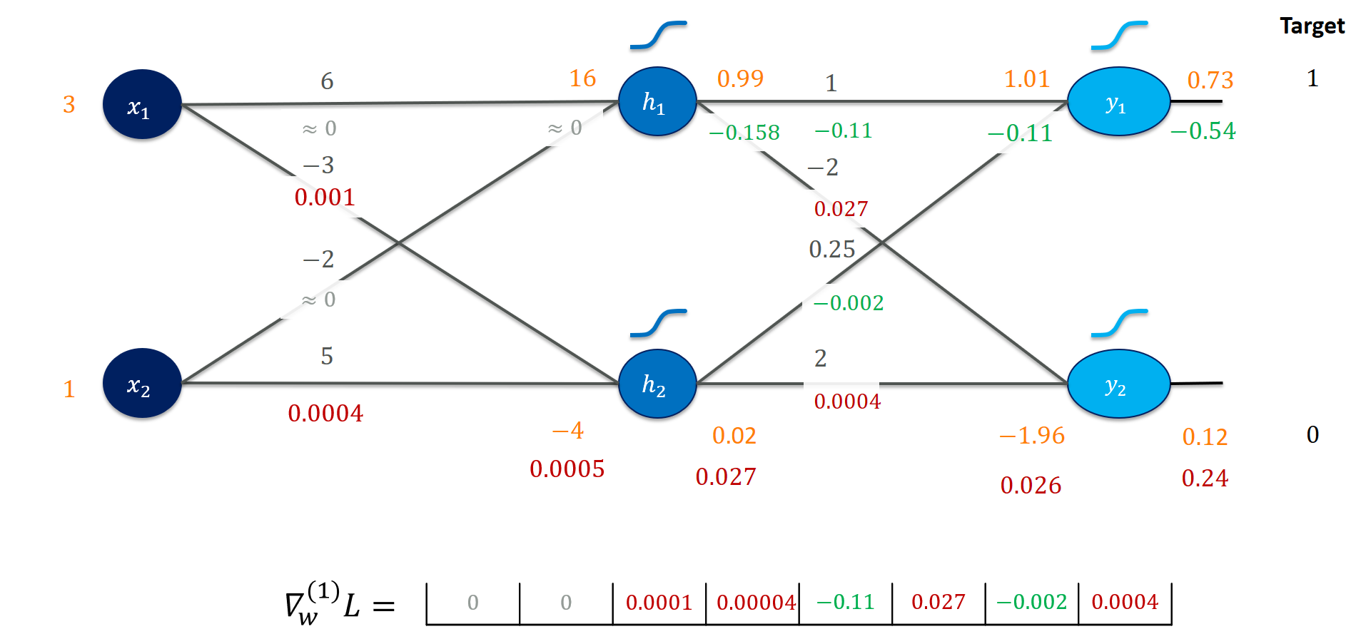
Algorithmic calculation using an autodiff system

That was somewhat tedious! Fortunately, you basically never have to do all of this work yourself. We can program classes for functions that know about the local derivatives and chain them together in a computational graph. Then we can automatically differentiate for the gradients. We’ll use the toy autodiff system from a previous post. To follow the code, every operation (e.g., multiply, sigmoid, add, etc.) becomes its own class that inherits from CompNode and is able to locally differentiate. A gradient tape is simply used as a log that protocols every operation in forward mode and plays it back when differentiating.

Here’s the network again:

gt = Tape()
# inputs, targets, and weights are our starting
# points
x1 = ConstantNode(3.,gt)
x2 = ConstantNode(1.,gt)

w11, w21 = ConstantNode(6.,gt), ConstantNode(-2.,gt)
w12, w22 = ConstantNode(-3.,gt), ConstantNode(5.,gt)

v11, v21 = ConstantNode(1.,gt), ConstantNode(0.25,gt)
v12, v22 = ConstantNode(-2.,gt), ConstantNode(2.,gt)

t1 = ConstantNode(1.,gt)
t2 = ConstantNode(0.,gt)

# calculating the hidden layer 
h1_in = Add(Multiply(x1, w11, gt), Multiply(x2, w21, gt), gt)
h2_in = Add(Multiply(x1, w12, gt), Multiply(x2, w22, gt), gt)
h1, h2 = Sigmoid(h1_in, gt), Sigmoid(h2_in, gt)

# calculating the output layer
y1_in = Add(Multiply(h1, v11, gt), Multiply(h2, v21, gt), gt)
y2_in = Add(Multiply(h1, v12, gt), Multiply(h2, v22, gt), gt)
y1, y2 = Sigmoid(y1_in, gt), Sigmoid(y2_in, gt)

t1_inv = Invert(t1, gt)
t2_inv = Invert(t2, gt)

e1 = Add(y1, t1_inv, gt)
e2 = Add(y2, t2_inv, gt)

l = Add(Square(e1, gt), Square(e2,gt), gt)
gt.forward()

You can imagine the syntax looking nicer if we used operator overloading to write e1 + e2 instead of Add(e1, e2). That’s what PyTorch and TensorFlow actually do. But I wanted to keep things explicit for learning the concepts.

Now the backward pass becomes rather easy and a quick check with our manual calculations shows everything went fine.

# now we can just play it backwards and inspect the results
gt.backward()

print("First layer gradients by framework")
print(w11.gradient, w12.gradient)
print(w21.gradient, w22.gradient)
>>> -5.34381483665323e-08 0.0014201436720081408
>>> -1.7812716122177433e-08 0.0004733812240027136
print("--")

print("First layer gradients manually")
print(grad_w11, grad_w12)
print(grad_w21, grad_w22)
>>> -5.34381483665323e-08 0.0014201436720081408
>>> -1.7812716122177433e-08 0.0004733812240027136

To inspect what’s going on “behind the scenes” (well, you actually know it after the manual steps anyway), I invite you to check out the Colab notebook:

Run in Google Colab

Although I certainly appreciate you playing around with the CompNode framework, I certainly would not expect anyone to use it as a starting point for productive applications. Therefore, let’s have a look at the same calculations using PyTorch:

import torch
x1 = torch.tensor(3., requires_grad=False)
x2 = torch.tensor(1., requires_grad=False)

w11 = torch.tensor(6., requires_grad=True)
w21 = torch.tensor(-2., requires_grad=True)
w12 = torch.tensor(-3., requires_grad=True)
w22 = torch.tensor(5., requires_grad=True)

v11 = torch.tensor(1., requires_grad=True)
v21 = torch.tensor(0.25, requires_grad=True)
v12 = torch.tensor(-2., requires_grad=True)
v22 = torch.tensor(2., requires_grad=True)

t1 = torch.tensor(1., requires_grad=False)
t2 = torch.tensor(0., requires_grad=False)

# calculating the hidden layer 
h1 = torch.sigmoid(w11*x1 + w21*x2)
h2 = torch.sigmoid(w12*x1 + w22*x2)

# calculating the output layer
y1 = torch.sigmoid(v11*h1 + v21*h2)
y2 = torch.sigmoid(v12*h1 + v22*h2)

e1 = y1 - t1
e2 = y2 - t2

# the loss function 
l = e1**2 + e2**2 

and again, this yields similar gradients:

l.backward()

print("First layer gradients by framework")
print(w11.grad, w12.grad)
print(w21.grad, w22.grad)
>>> tensor(-5.6607e-08) tensor(0.0014)
>>> tensor(-1.8869e-08) tensor(0.0005)

print("First layer gradients manually")
print(grad_w11, grad_w12)
print(grad_w21, grad_w22)
>>> -5.34381483665323e-08 0.0014201436720081408
>>> -1.7812716122177433e-08 0.0004733812240027136

The small differences result from rounding errors since PyTorch uses 32-bit floats as default in contrast to 64-bit floats (doubles) in Numpy. Changing this explicitly to, e.g.,

x1 = torch.tensor(3., requires_grad=False,dtype=torch.float64)

alleviates this problem:

>>> tensor(-5.3438e-08, dtype=torch.float64) tensor(0.0014, dtype=torch.float64)
>>> tensor(-1.7813e-08, dtype=torch.float64) tensor(0.0005, dtype=torch.float64)

You should never actually write productive code like this in PyTorch! The elementary unit is a tensor, i.e., a multidimensional array and vectorized operations can take advantage of GPU-acceleration. Moreover, many convenience abstractions such as layers, loss functions, or optimizers are handily available in PyTorch. This example lets us peek under the hood.

Vectorized implementation using matrices

Most importantly, we will look at a vectorized implementation for our neural network next. In essence, all of the weighted sums (aka dot-products between inputs and weights) will be summarized in matrix multiplications. Consider the following video clip for an animated overview:

Every training instance becomes a row in a matrix $X$. Every column corresponds to one input feature. We apply a weight matrix $W$ simply by matrix multiplication: $H = XW$. Here, each column of $W$ contains the weights for one hidden unit. Every row of $H$ still corresponds to the the respective input.

# first, the training data (for now, just one instance) 
X = np.array( [[3., 1. ]])
T = np.array( [[1., 0. ]])

# then the weights 
W = np.array([[6., -3.], [-2., 5.]])
V = np.array([[1., -2.], [0.25, 2.]])

# now the forward pass 
H_in = np.dot(X,W)
H = sigmoid(H_in)
# ---- 
Y_in = np.dot(H,V)
Y = sigmoid(Y_in)
print(Y)
>>> [[0.73194171 0.12303186]]

That looks familiar! Using operations from linear algebra such as matrix multiplications helped us hide a lot of the underlying complexity of a neural network. In particular, imagine increasing the number of hidden units you’d like your network to have, say five instead of two. Simply adapt the dimensions of $W$ (how?).

Let’s calculate the loss function per training instance next:

# now for the loss function per training instance
# simply apply componentwise subtraction
E = Y - T 
# square each term
E_sq = E**2
# sum up per row (keep dimensions as they are)
L = np.sum(E_sq, axis=1, keepdims=True)
print(L)
>>> [[0.08699208]] 

Now, what about the gradients? The shortcut would be now to just use PyTorch again …

If we want to work it out using plain numpy, we could now dive deep into matrix calculus, the chain rule for matrix-vector products etc. or we just work out the operations based on their scalar counterparts. Don’t get me wrong, I think the topic is really useful and Deisenroth, Faisal, and Ong do a really fine job explaining it. But for our purposes we can get away with very little of that.

Let me just state a couple of facts I found useful:

• Differentiating a function with respect to a vector simply means taking each dimension’s partial derivative in isolation and bringing them back to vector form. The same basically applies to matrices and tensors.
• If you have a function $f$ with $m$ inputs $(x_1, \ldots, x_m)$ and $n$ outputs $(y_1, \ldots, y_n)$ (i.e., it is vector-valued), you have $m \cdot n$ ways of taking a derivative. For instance, how does output $y_4$ change when you increase $x_2$ etc. Stack those entries in a nice matrix and you get the Jacobian.
• Vectors, matrices, and tensors do not really add any new complexity to differentiation other than keeping things in a grid.
• There are nice extensions of the scalar calculus rules (sum rule, product rule, chain rule) to the vector case. That makes them suitable for CompNode implementations.

Again, we get away with just directly approaching our task. First, let’s find the gradients before and after the output sigmoid activation. These are simply componentwise calculations.

grad_Y = 2*E
grad_Y_in = (Y) * (1-Y) * grad_Y
print(grad_Y_in)
>>> [[-0.1051877   0.02654905]]

Those values look familiar:

Next, let’s work out the gradients for the weights $V$. Zoom in on the weights again:

Generalizing from that example a little bit:

\[\frac{\partial L}{ \partial v_{i,j}} = \frac{\partial L}{\partial y_j^{(\mathit{in})}} \cdot \underbrace{ \frac{\partial y_j^{(\mathit{in})}}{\partial v_{i,j}} }_{h_i}\]

Hence, the gradient of the $(i,j)$-th entry of the weight matrix $V$ is simply the product of $h_i$ and $(\frac{\partial L}{\partial \vec{y}^{(\mathit{in})}})_j$ that we already stored in grad_Y_in. Given both h and grad_Y_in as $(1 \times 2)$-vectors, how could you achieve a matrix that has the appropriate entries?

A nice “trick” to get exactly these quantities for a grad_V matrix is by performing the outer product of our vectors H and grad_Y_in, i.e., multiplying a column vector $(n \times 1)$ with a row vector $(1 \times m)$ for form a $(n \times m)$-matrix. Since we stored H as a row vector, we need to transpose it first.

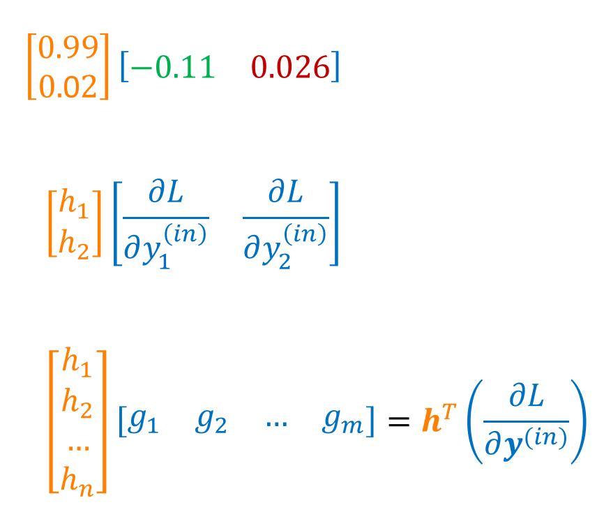
The according code is very concise and hides all of that away:

grad_V = np.dot(H.T, grad_Y_in)
print(grad_V)
>>> [[-0.10518769  0.02654905]
>>>  [-0.00189193  0.00047752]]

Finally, let’s work our way to the hidden outputs, recall:

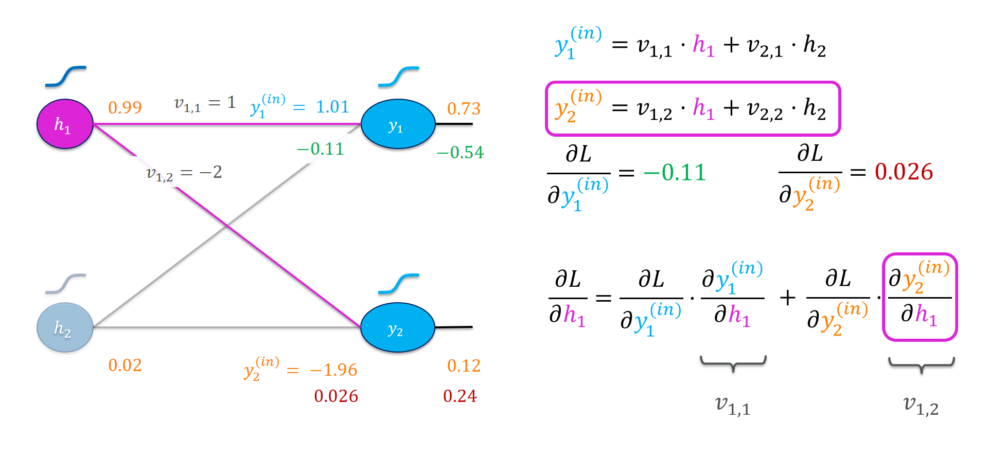
Again, let us generalize a little bit from that example. We look for the derivative of the loss with respect to the $i$-th entry of $\vec{h}$.

\[\frac{\partial L}{ \partial h_{i}} = \frac{\partial L}{\partial y_1^{(\mathit{in})}} \cdot \underbrace{ \frac{\partial y_1^{(\mathit{in})}}{\partial h_{i}} }_{v_{i,1}} + \frac{\partial L}{\partial y_2^{(\mathit{in})}} \cdot \underbrace{ \frac{\partial y_2^{(\mathit{in})}}{\partial h_{i}} }_{v_{i,2}} = \sum_{j = 1}^{2} \frac{\partial L}{\partial y_j^{(\mathit{in})}} \cdot v_{i, j}\]

Remember that this calculation basically uses the weight matrix “in reverse”. It calculates a weighted sum of all the gradients of the outgoing nodes.

Our hidden output gradient will be a $(1 \times m)$-row vector where $m$ is the number of hidden units (here, $h = 2$). Every entry $\frac{\partial L}{ \partial h_{i}}$ is a dot-product between the output gradient $\frac{\partial L}{\partial \vec{y}^{(\mathit{in})}}$ and the $i$-row of the matrix $V$. To align this with matrix multiplication, we can simply transpose $V$ to get each row as a column to multiply with.

grad_H = np.dot(grad_Y_in, V.T)
print(grad_H)
>>> [[-0.1582858   0.02680117]]

That again looks familiar! Now our job is complete for a single layer and we need to apply exactly the same steps again for the hidden layer:

# now on to the hidden layer
grad_H_in = (H * (1.-H))*grad_H # sigmoid
grad_W = np.dot(X.T, grad_H_in) # outer product
grad_X = np.dot(grad_H_in, W.T) # not really necessary
print(grad_W)
>>> [[-5.34381484e-08  1.42014367e-03]
>>> [-1.78127161e-08  4.73381224e-04]]

We have seen these gradients before! We’re now ready to wrap this up in a nice class:

import numpy as np

def sigmoid(z):
    return 1./(1. + np.exp(-z))

class NeuralNetwork:
    def __init__(self, input_dim=2, hidden_dim=2, output_dim=2):
        self.W = 0.1 * np.random.rand(input_dim, hidden_dim)
        self.V = 0.1 * np.random.rand(hidden_dim, output_dim)
                
    # expects X to be a (n X input_dim) matrix
    def forward(self, X):
        self.X = X # keep for backward pass 
        
        self.H_in = np.dot(X, self.W)
        self.H = sigmoid(self.H_in)
        # ---- 
        self.Y_in = np.dot(self.H, self.V)
        self.Y = sigmoid(self.Y_in)
        return self.Y
    
    # expects T to be a (n X output_dim) matrix 
    def backward(self, T):
        E = self.Y - T 
        E_sq = E**2
        self.L = np.sum(E_sq, axis=1, keepdims=True)
        grad_Y = 2*E
        
        # -----
        grad_Y_in = (self.Y) * (1-self.Y) * grad_Y # sigmoid
        grad_V = np.dot(self.H.T, grad_Y_in) # outer product
        grad_H = np.dot(grad_Y_in, self.V.T)
        
        # -----
        grad_H_in = (self.H * (1.-self.H))*grad_H # sigmoid
        grad_W = np.dot(self.X.T, grad_H_in) # outer product
        return grad_W, grad_V

and a quick test case confirms that everything worked fine:

net = NeuralNetwork()
net.W, net.V = W, V
net.forward(X)
g_W, g_V = net.backward(T)
print(g_W)
print(g_V)
>>> [[-5.34381484e-08  1.42014367e-03]
>>>  [-1.78127161e-08  4.73381224e-04]]
>>> [[-0.10518769  0.02654905]
>>>  [-0.00189193  0.00047752]]

Finally, we have a concise and encapsulated way of calculating the gradients for a simple feedforward network. Let’s now apply those gradients to see if we can improve the performance of the network.

Applying the gradient updates

Determining the partial derivatives of the loss function with respect to the weights is only half of the story. We interpret them as “weight change requests”. Now it’s time to actually do that. Our NeuralNetwork class provides a convenient abstraction to get the gradients such that we can write up a little training loop.

But let’s do this step by step. Recall that we have a training set consisting of two instances.

First, we get the gradients for both training instances.

net = NeuralNetwork()

net.W = W.copy()
net.V = V.copy()

# first training instance
X = np.array( [[3., 1. ]])
T = np.array( [[1., 0. ]])
net.forward(X)
g_W_1, g_V_1 = net.backward(T)
# initial loss
init_loss_1 = net.L

# second training instance
X = np.array( [[-1., 4. ]])
T = np.array( [[0., 1. ]])
net.forward(X)
g_W_2, g_V_2 = net.backward(T)
# initial loss
init_loss_2 = net.L

g_W, g_V = g_W_1 + g_W_2, g_V_1 + g_V_2

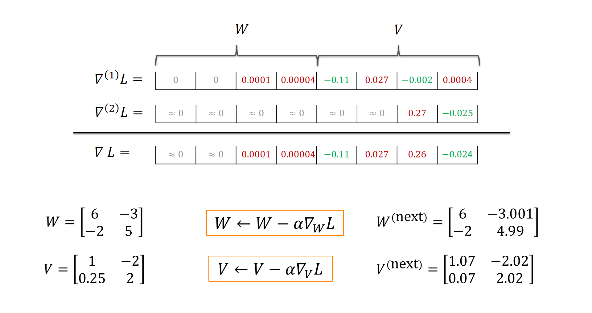
Each training instance has its own “suggestions” as to how to adapt the weights $W$ and $V$. For instance, training instance 1 “suggests” that $V_{2,2}$ be decreased (the loss increases with rising $V_{2,2}$ by a factor of 0.0004) whereas training instance 2 predicts a loss decrease by a factor of -0.025 if we increase $V_{2,2}$. Taking the sum or average makes sure that we get an overall loss gradient that is assumed to reduce the overall loss the most. Here, training instance is responsible for increasing $V_{2,2}$. You can view this as kind of a “compromise” that reduces overfitting to single instances. With that overall loss gradient, we can apply the weight update:

# update weights
alpha = 0.5 # very large for demonstration

net.W -= alpha * g_W
net.V -= alpha * g_V

print(net.V)
>>> [[ 1.06837185 -2.01725687]
>>>  [ 0.07134767  2.01595986]]

Indeed, $V_{2,2}$ has increased, for example. But did that help our performance on the training set?

Let’s inspect the first instance:

X = np.array( [[3., 1. ]])
T = np.array( [[1., 0. ]])
y = net.forward(X)
print(y)
>>> [[0.74165987 0.12162137]]

Well, that looks promising! The target value would be $(1,0)$ and we moved $y_1$ closer to $1$ and $y_2$ closer to $0$. Closer inspection shows the changes the gradient update provoked (for example, weighting the output $h_1$ higher for $y_1$ leads to a higher output score in $y_1$):

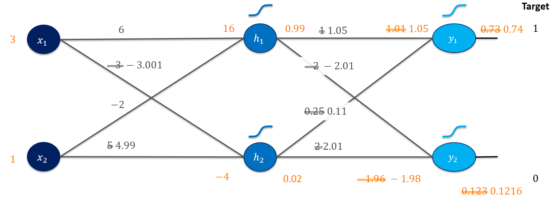
Is this reflected in our loss?

net.backward(T)
print("Old loss for instance #1:", init_loss_1)
print("New loss for instance #1:", net.L)
>>> Old loss for instance #1: [[0.08699208]]
>>> New loss for instance #1: [[0.08153138]]

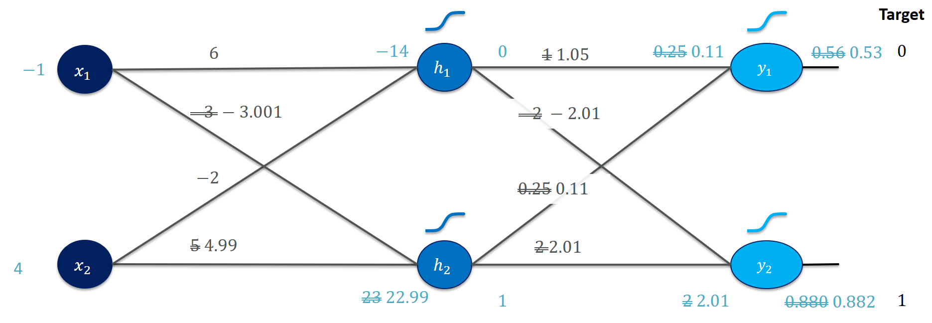
That looks good! Can we observe similar improvements for the second training example?

X = np.array( [[-1., 4. ]])
T = np.array( [[0., 1. ]])
y = net.forward(X)
print(y)
>>> [[0.52811432 0.88207988]]

net.backward(T)
print("Old loss for instance #2:", init_loss_2)
print("New loss for instance #2:", net.L)
>>> Old loss for instance #2: [[0.33025203]]
>>> New loss for instance #2: [[0.29280989]]

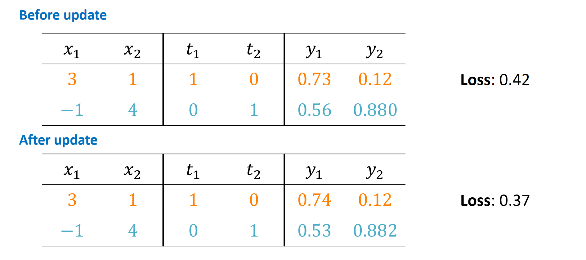
Or, more visually,

where we can see that the updated weights $W$ and $V$ helped matching the target values better (also reflected in the loss).

This simple example sneaked in a little complication that is frequently incurred in training neural networks: vanishing gradients. Almost no changes were made to the weights $W$ of the hidden layer. The increased performance is almost exclusively due to the adapted weights $V$ in the output layer.

If we inspect the gradients for the weights $W$ of the hidden layer more closely

print(grad_W)
>>> [[-5.34381484e-08  1.42014367e-03]
>>>  [-1.78127161e-08  4.73381224e-04]]

we notice that the magnitude of the gradients is very small, almost 0. The main culprit here is the activation function sigmoid which flattens out at inputs such as $16$. You could also say that our initially chosen weights (6, -2, …) are ridiculously high. And you would never start training like that. That is where proper initialization such as He or Xavier come into play. Also, batch normalization helps here (try to implement it for the two instance training set).

Let’s inspect the effects of our gradient update in one picture:

In a productive setting, you would see loss curves (e.g., in TensorBoard) that do not care about a single update step but plot the results of many, many steps over time versus the overall training loss. You would hope to see that curve going down to a very low value for the training loss – without overfitting (but that’s another topic).

Finally, let’s see what happens to the weights if we continue training (just with these two instances) for 200 epochs:

# iterate for 200 epochs
train_X = np.array( [[3., 1. ], [-1., 4.]])
train_T = np.array( [[1., 0. ], [0., 1.]])

n_epochs = 200
alpha = 0.5

for n in range(n_epochs):
    # grad_W
    grad_W = np.zeros_like(net.W)
    grad_V = np.zeros_like(net.V)
    for i in range(train_X.shape[0]):
        X = train_X[i, :].reshape(1,-1)
        T = train_T[i, :].reshape(1,-1)
        
        net.forward(X)
        grad_W_i, grad_V_i = net.backward(T)
        grad_W += grad_W_i
        grad_V += grad_V_i
    
    # apply gradient 
    net.W -= alpha * grad_W
    net.V -= alpha * grad_V
    
# inspect the trained net's outputs
print(net.forward(np.array([3.,1.])))
print(net.forward(np.array([-1.,4.])))
>>> [0.94607312 0.04903031]
>>> [0.05606368 0.95082381]

We ended up adapting the weights $W$ and $V$ in a way that classifies both instances very well. But what do the weights look like now?

While we observe that the weights $V$ are now substantially different from where we started, also the weights in $W$ did change a little bit. Of course, our example with two training instances is silly and it’s no miracle that we can fit a net to classify these well. However, it contains all essential steps of backpropagation and we could go on to train more realistic nets. I’d suggest looking at Karpathy’s minimal neural network example next. I implemented an object-oriented version of it at:

Run in Google Colab

This simple net can be used for many interesting things. Grad a dataset such as MNIST or Fashion-MNIST and play around with it.

Conclusion

We worked through all backpropagation steps for a concrete 2-2-2 neural network, gradient calculations and weight updates. The calculus business can, in principle, be done manually or left to an automatic differentiation system. Essentially, the chain rule is worked out in a way that maximizes reuse of downstream gradients which saves redundant calculations. A lot of the complexity is hidden behind linear algebra expressions. They are certainly really useful (also for GPU acceleration) but it pays off to be aware of what you’re working with. I really hope this example was as useful to you as it was for me during writing.